Plot ELPI data

First we import the aerosoltools package

import aerosoltools as at;

Next we import the ELPI data via the Load function. The filename variable should give the path and filename of the relevant dataset.

filename = r"..\..\..\tests\data\Sample_ELPI.txt";
ELPI_data = at.Load_ELPI_file(filename);

The data is now loaded and can be treated or plotted directly.

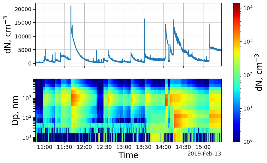
A quick way to visualize the data is via a timeseries plot, which can be done with a single line of code, as seen below. Here it is important to note, that the keyword y_3d is used to give a lower bound of 1 for the logarithmic colorbar. This was needed as some concentrations were reported as 0, which cannot be shown on a log scale.

ELPI_data.plot_timeseries(y_3d=(1,0));

Check Various metadata

We can also check various metadata loaded directly from the elpi data file

# We can check the unit of the data. All load functions return number concentration data also if the original data file was in a different mode
print(ELPI_data.unit)

cm$^{-3}$

# We can check the data type
print(ELPI_data.dtype)

dN

# We can ensure that the correct instrument was stored
print(ELPI_data.instrument)

ELPI

# We can check the density of the datafile, which should always be given in g/cm3
print(ELPI_data.density)

1.0