Activities, peaks, and exposure statistics
This example shows how to:
Load a 1D time series (CPC total number concentration)
Inspect main and extra data
Define simple time segments (activities)
Detect peaks using
Peak_finderPlot total concentration with activity shading
Summarize activities and compute exposure metrics with
summarize_exposure
[ ]:
import matplotlib.pyplot as plt
import aerosoltools as at
Load CPC sample data
Here we load a sample CPC file from the test data folder. Adjust the path if you keep example data elsewhere.
[2]:
filename = r"..\..\tests\data\Sample_CPC_AIM.txt"
cpc = at.Load_CPC_file(filename,extra_data=True)
Inspect metadata and extra data
The loader returns an Aerosol1D instance with:
.data– main time series + activity masks.extra_data– optional additional channels (environmental, meta, etc.).metadata– instrument, unit, etc.
[26]:
print("Metadata:\n", cpc.metadata)
print("\nMain columns:", list(cpc.data.columns))
print("Extra-data columns:", list(cpc.extra_data.columns))
Metadata:
 {'instrument': 'CPC', 'serial_number': '06160001 ', 'unit': 'cm$^{-3}$'}

Main columns: ['Total_conc', 'All data']
Extra-data columns: ['Sample Length (s)', 'Averaging Interval (s)', 'Title', 'Instrument ID', 'Instrument Errors', 'Mean(#/cm³)', 'Min(#/cm³)', 'Max(#/cm³)', 'Std. Dev.(#/cm³)', 'Comments']
You can access data in the main DataFrame via the .data property of the defined cpc variable:
[27]:
cpc.data
[27]:
| Total_conc | All data | |
|---|---|---|
| Datetime | ||
| 2023-08-14 11:14:29 | 1468 | True |
| 2023-08-14 11:14:30 | 1459 | True |
| 2023-08-14 11:14:31 | 1437 | True |
| 2023-08-14 11:14:32 | 1462 | True |
| 2023-08-14 11:14:33 | 1481 | True |
| ... | ... | ... |
| 2023-08-14 11:20:49 | 1293 | True |
| 2023-08-14 11:20:50 | 1307 | True |
| 2023-08-14 11:20:51 | 1311 | True |
| 2023-08-14 11:20:52 | 1295 | True |
| 2023-08-14 11:20:53 | 1311 | True |
384 rows × 2 columns
Similarly, you can access any additional data columns extracted from the raw data via the .extra_data property:
[28]:
cpc.extra_data
[28]:
| Sample Length (s) | Averaging Interval (s) | Title | Instrument ID | Instrument Errors | Mean(#/cm³) | Min(#/cm³) | Max(#/cm³) | Std. Dev.(#/cm³) | Comments | |
|---|---|---|---|---|---|---|---|---|---|---|
| Datetime | ||||||||||
| 2023-08-14 11:14:29 | 00:01 | 1 | 3007-06160001 3.1 | NaN | 1468 | 1468 | 1468 | 0 | NaN | |
| 2023-08-14 11:14:30 | 00:01 | 1 | 3007-06160001 3.1 | NaN | 1459 | 1459 | 1459 | 0 | NaN | |
| 2023-08-14 11:14:31 | 00:01 | 1 | 3007-06160001 3.1 | NaN | 1437 | 1437 | 1437 | 0 | NaN | |
| 2023-08-14 11:14:32 | 00:01 | 1 | 3007-06160001 3.1 | NaN | 1462 | 1462 | 1462 | 0 | NaN | |
| 2023-08-14 11:14:33 | 00:01 | 1 | 3007-06160001 3.1 | NaN | 1481 | 1481 | 1481 | 0 | NaN | |
| ... | ... | ... | ... | ... | ... | ... | ... | ... | ... | ... |
| 2023-08-14 11:20:49 | 00:01 | 1 | 3007-06160001 3.1 | NaN | 1293 | 1293 | 1293 | 0 | NaN | |
| 2023-08-14 11:20:50 | 00:01 | 1 | 3007-06160001 3.1 | NaN | 1307 | 1307 | 1307 | 0 | NaN | |
| 2023-08-14 11:20:51 | 00:01 | 1 | 3007-06160001 3.1 | NaN | 1311 | 1311 | 1311 | 0 | NaN | |
| 2023-08-14 11:20:52 | 00:01 | 1 | 3007-06160001 3.1 | NaN | 1295 | 1295 | 1295 | 0 | NaN | |
| 2023-08-14 11:20:53 | 00:01 | 1 | 3007-06160001 3.1 | NaN | 1311 | 1311 | 1311 | 0 | NaN |
384 rows × 10 columns
Plot total concentration
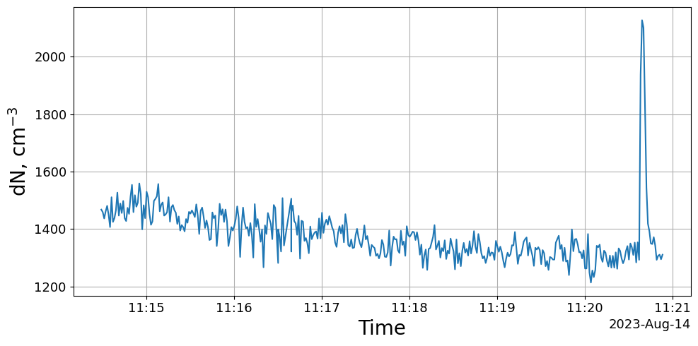
Use plot_total_conc() to quickly visualize the time series.
[3]:
cpc.plot_total_conc()
[3]:
(<Figure size 1000x500 with 1 Axes>,
 <Axes: xlabel='Time', ylabel='dN, cm$^{-3}$'>)
Detect peaks with Peak_finder
Peak_finder flags time steps where the signal exceeds a rolling baseline by more than ratio * rolling_std. The resulting mask is stored as the "Peak" activity.
[5]:
cpc.Peak_finder(window=15, ratio=2.5, method="median")
cpc.activities
[5]:
['All data', 'Peak']
We can also mark specific activities based on timestamps:
[11]:
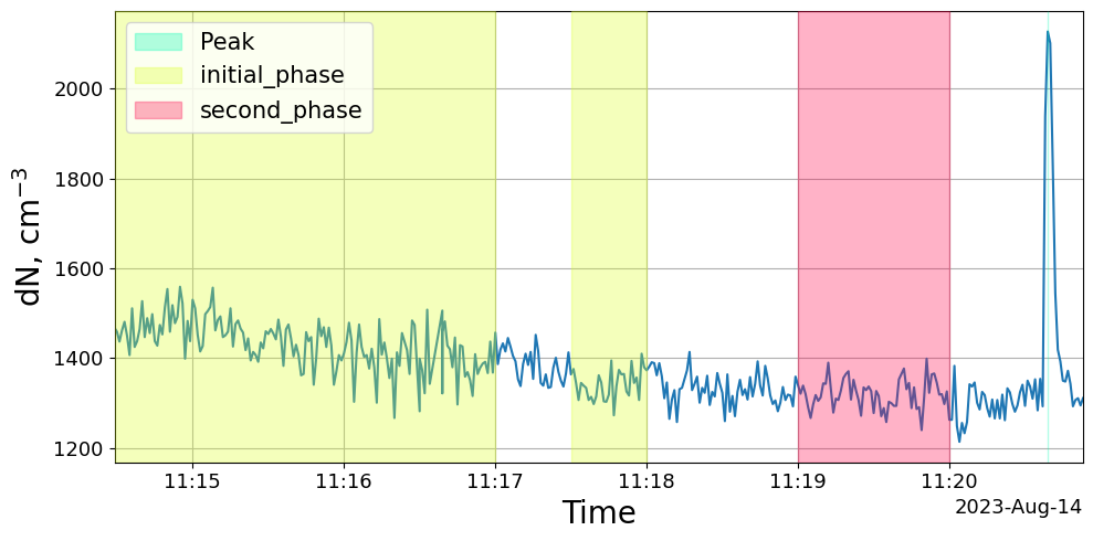
activity_periods= {
    "initial_phase": [
        ("2023-08-14 11:14:00", "2023-08-14 11:17:00"),
        ("2023-08-14 11:17:30", "2023-08-14 11:18:00")],
    "second_phase": [
        ("2023-08-14 11:19:00", "2023-08-14 11:20:00")]
}
cpc.mark_activities(activity_periods)
Plot with activity shading
We can overlay activities (including the automatically created "Peak" mask) on top of the total concentration time series.
[12]:
cpc.plot_total_conc(mark_activities=True)
[12]:
(<Figure size 1000x500 with 1 Axes>,
 <Axes: xlabel='Time', ylabel='dN, cm$^{-3}$'>)
Summarize activities
summarize_activities() reports basic descriptive statistics per activity, including duration, mean, median, and number of samples.
[13]:
cpc.summarize_activities()
Summary of total concentration per activity:

+--------------------+----------+--------+---------------+--------------+
|    Metric/Field    | All data |  Peak  | initial_phase | second_phase |
+--------------------+----------+--------+---------------+--------------+
|   Duration (min)   |  6.417   | 0.017  |     3.05      |    1.017     |
|  Duration (HH:MM)  |  00:06   | 00:00  |     00:03     |    00:01     |
|  Min (cm$^{-3}$)   |  1214.0  | 2127.0 |    1267.0     |    1240.0    |
|  Max (cm$^{-3}$)   |  2127.0  | 2127.0 |    1559.0     |    1399.0    |
|  Mean (cm$^{-3}$)  | 1379.339 | 2127.0 |   1417.346    |   1319.869   |
| Median (cm$^{-3}$) |  1364.0  | 2127.0 |    1425.0     |    1320.0    |
|  Std (cm$^{-3}$)   |  94.659  |  nan   |    62.829     |    33.21     |
|     N samples      |   384    |   1    |      182      |      61      |
+--------------------+----------+--------+---------------+--------------+
[13]:
| Segment | Duration (min) | Duration (HH:MM) | Min (cm$^{-3}$) | Max (cm$^{-3}$) | Mean (cm$^{-3}$) | Median (cm$^{-3}$) | Std (cm$^{-3}$) | N samples | |
|---|---|---|---|---|---|---|---|---|---|
| 0 | All data | 6.417 | 00:06 | 1214.0 | 2127.0 | 1379.339 | 1364.0 | 94.659 | 384 |
| 1 | Peak | 0.017 | 00:00 | 2127.0 | 2127.0 | 2127.000 | 2127.0 | NaN | 1 |
| 2 | initial_phase | 3.050 | 00:03 | 1267.0 | 1559.0 | 1417.346 | 1425.0 | 62.829 | 182 |
| 3 | second_phase | 1.017 | 00:01 | 1240.0 | 1399.0 | 1319.869 | 1320.0 | 33.210 | 61 |
Exposure summary for PNC
Finally, we use summarize_exposure on the Aerosol1D object to compute exposure metrics for total number concentration (PNC):
duration, mean, percentiles
time above a long-term limit
short-term (window-based) exceedances
an 8-hour TWA (by default)
[14]:
exp = cpc.summarize_exposure(
    metric="PNC",           # use total_concentration
    activity="All data",    # summarize whole record
    background=None,        # assume zero background outside the record
    exposure_hours=8.0,     # Set how long a worker was exposed to the measured concentration
    short_limit=1.0,        # Short term exposure limit for the given metric (if available)
    long_limit=1.0,         # long term or 8hr exposure limit for the given metric
    short_window="15min",   # Length of short term exposures to identify
)
exp
Exposure summary for activity 'All data' and metric 'PNC' (cm$^{-3}$):

+--------------------------------------------+-----------+
|                   Field                    |   Value   |
+--------------------------------------------+-----------+
|                   Metric                   |    PNC    |
|                    Unit                    | cm$^{-3}$ |
|                  Samples                   |    384    |
|                Duration_min                |   6.42    |
|               Duration_HH:MM               |   00:06   |
|                    Mean                    | 1379.018  |
|                    Std                     |  94.659   |
|                   Median                   |  1364.0   |
|                    Max                     |  2127.0   |
|                  Seg_TWA                   | 1379.018  |
|                 Window_TWA                 | 1379.018  |
|             Window_TWA_window              |    8h     |
|                Short_limit                 |    1.0    |
|                Short_window                |   15min   |
|         Short_limit_exceedance_min         |   6.42    |
|      Short_limit_exceedance_fraction       |    1.0    |
|   Short_limit_fullwindow_exceedance_min    |   0.02    |
| Short_limit_fullwindow_exceedance_episodes |     1     |
|                 Long_limit                 |    1.0    |
|            Long_limit_exceeded             |   True    |
|         Long_limit_exceedance_min          |   6.42    |
|                    C95                     |  1503.95  |
|                    C99                     |  1605.24  |
|                    IQR                     |  107.25   |
|                   Peaks                    |     1     |
+--------------------------------------------+-----------+
[14]:
| Segment | Metric | Unit | Samples | Duration_min | Duration_HH:MM | Mean | Std | Median | Max | ... | Short_limit_exceedance_fraction | Short_limit_fullwindow_exceedance_min | Short_limit_fullwindow_exceedance_episodes | Long_limit | Long_limit_exceeded | Long_limit_exceedance_min | C95 | C99 | IQR | Peaks | |
|---|---|---|---|---|---|---|---|---|---|---|---|---|---|---|---|---|---|---|---|---|---|
| 0 | All data | PNC | cm$^{-3}$ | 384 | 6.42 | 00:06 | 1379.018 | 94.659 | 1364.0 | 2127.0 | ... | 1.0 | 0.02 | 1 | 1.0 | True | 6.42 | 1503.95 | 1605.24 | 107.25 | 1 |
1 rows × 26 columns