Combine NS+OPS and extra_data

This example illustrates how to:

• Load data from two different instruments (NS and OPS)

• Combine them on a common time base

• Inspect and use the extra_data tables

import matplotlib.pyplot as plt
import aerosoltools as at

Load NS and OPS datasets

A sample NanoScan (NS) and several OPS files are included in the test data directory. Here we utilize the very efficient Load_data_from_folder function, which can load and combine multiple files from the same instrument, by specifying a path and the loader function to use. In this example we also specify a (optional) search_word, which can be used to load only files containing this specific keyword in their name.

ns_file = r"..\..\tests\data\Combine_example_NS.csv"
ops_path = r"..\..\tests\data"

ns = at.Load_NS_file(ns_file, extra_data  =True)
ops = at.Load_data_from_folder(ops_path, at.Load_OPS_file, search_word="Combine_example",extra_data=True)

File load summary:

+----------------------------------+---------+------------------------------------------------------------------------------------+
|               File               | Status  |                                       Reason                                       |
+----------------------------------+---------+------------------------------------------------------------------------------------+
| Combine_example_OPS - file 1.csv | Loaded  |                                         -                                          |
| Combine_example_OPS - file 2.csv | Loaded  |                                         -                                          |
| Combine_example_OPS - file 3.csv | Loaded  |                                         -                                          |
| Combine_example_OPS - file 4.csv | Loaded  |                                         -                                          |
|      Combine_example_NS.csv      | Skipped | IndexError: too many indices for array: array is 0-dimensional, but 1 were indexed |
+----------------------------------+---------+------------------------------------------------------------------------------------+

The Load_data_from_folder function displays a progress bar so you can see how many files are loaded and the progress. In addition it prints a summary table, listing the files that were loaded, those that were skipped, and a reason as to why these were skipped.

This enables you to load many files from a folder, which can include from subfolders, even if the folder contains many different files, where a simple search_word cannot distinguish them efficiently.

Inspect extra_data for each instrument

Many loaders store auxiliary variables (e.g. flow, temperature, status flags) in the .extra_data attribute.

print("NS extra-data columns:", list(ns.extra_data.columns))
print("OPS extra-data columns:", list(ops.extra_data.columns))

# Show a small snippet if available
display(ns.extra_data.head())
display(ops.extra_data.head())

NS extra-data columns: ['Median (nm)', 'Mean (nm)', 'Geo Mean (nm)', 'Mode (nm)', 'GSD', 'Particle Density (g/cc)', 'Firmware Version', 'Status']
OPS extra-data columns: ['Bin 1', 'Deadtime (s)', 'Temperature (C)', 'Humidity (%)', 'Ambient Pressure (kPa)', 'Alarms', 'Errors', 'Unnamed: 24']

	Median (nm)	Mean (nm)	Geo Mean (nm)	Mode (nm)	GSD	Particle Density (g/cc)	Firmware Version	Status
Datetime
2023-05-30 15:41:29	15.7036	25.3091	18.5497	15.3993	1.8865	1.0	1.4	Filling reservoir;
2023-05-30 15:42:29	16.7808	29.9378	21.1565	15.3993	2.0303	1.0	1.4	No errors
2023-05-30 15:43:29	15.6058	21.0331	17.1038	15.3993	1.6626	1.0	1.4	Filling reservoir;
2023-05-30 15:44:29	15.7465	21.2670	17.2874	15.3993	1.6668	1.0	1.4	No errors
2023-05-30 15:45:29	16.3273	24.3266	18.8023	15.3993	1.7967	1.0	1.4	No errors

	Bin 1	Deadtime (s)	Temperature (C)	Humidity (%)	Ambient Pressure (kPa)	Alarms	Errors	Unnamed: 24
Datetime
2023-10-23 13:30:44	0	0.000000	30.668	0.0	100.739	NaN	NaN	NaN
2023-10-23 13:31:44	144	0.007004	30.724	0.0	100.733	NaN	NaN	NaN
2023-10-23 13:32:44	2186	0.103820	30.804	0.0	100.732	NaN	NaN	NaN
2023-10-23 13:33:44	0	0.000000	30.867	0.0	100.733	NaN	NaN	NaN
2023-10-23 13:34:44	0	0.000000	30.932	0.0	100.729	NaN	NaN	NaN

Combine NS and OPS on a common time grid

The helper function Combine_NS_OPS aligns the two instruments in time and returns a combined dataset suitable for correlation analysis. If the timestamps between the two datasets does not match precisely e.g. differ a few seconds, then the matching can be relaxed via the match keyword. This can be set to either nearest, matching nearest datapoint within a tolerance time window.

If the two datasets do not have the same sampling frequency e.g. one is per minute and the other is every second, the function can be called with match = "rebin", rebin_freq = "1min", in which case the high frequency data is rebinned into 1 min times to match the low frequency data. A larger and common frequency can also be set.

combined = at.Combine_NS_OPS(ns, ops, match="nearest",tolerance="30s",)
combined.data

	Total_conc	11.5	15.4	20.5	27.4	36.5	48.7	64.9	86.6	115.5	...	1561.5	1944.0	2420.5	3014.0	3752.5	4672.0	5816.5	7241.0	9015.5	All data
Datetime
2023-10-23 13:31:19	28754.398451	1485.4313	3835.8508	4568.8809	5940.7231	5474.6567	3735.8103	1953.4159	1017.3690	560.3550	...	0.052996	0.035997	0.026998	0.024998	0.013999	0.006000	0.006000	0.002000	0.004000	True
2023-10-23 13:32:19	28443.038346	1638.4261	3983.9104	4449.2646	5711.5151	5321.5229	3699.7014	1971.2294	1002.8712	513.6530	...	0.547839	0.462708	0.430659	0.332509	0.221339	0.110169	0.081124	0.055084	0.055084	True
2023-10-23 13:33:19	28263.426000	1432.7457	3766.0723	4466.9683	5829.9810	5441.0298	3779.6973	2001.2233	994.9397	468.5747	...	0.000000	0.000000	0.000000	0.000000	0.000000	0.000000	0.000000	0.000000	0.000000	True
2023-10-23 13:34:19	27502.510700	1694.3612	3835.4392	4182.8892	5507.8789	5217.7969	3656.2771	1933.9193	948.3063	440.3977	...	0.000000	0.000000	0.000000	0.000000	0.000000	0.000000	0.000000	0.000000	0.000000	True
2023-10-23 13:35:19	28912.922700	1746.8145	3937.4988	4386.7480	5792.1016	5432.0537	3771.3831	2020.9584	1083.6498	585.2220	...	0.000000	0.000000	0.000000	0.000000	0.000000	0.000000	0.000000	0.000000	0.000000	True
...	...	...	...	...	...	...	...	...	...	...	...	...	...	...	...	...	...	...	...	...	...
2023-10-26 23:22:58	10894.390593	566.0240	1299.7166	1351.1873	2046.0566	2273.6438	1849.0562	1053.4200	357.7328	0.0000	...	2.181798	1.857042	1.711253	1.462910	0.872719	0.421278	0.319729	0.257392	0.282528	True
2023-10-26 23:23:58	10677.534091	521.8893	1213.6832	1371.0192	1979.4780	2195.3396	1825.7404	1096.6410	402.9259	0.0000	...	1.891105	1.637886	1.498213	1.254038	0.832006	0.356717	0.293413	0.204987	0.275326	True
2023-10-26 23:24:58	10860.292970	610.1611	1343.8060	1359.7363	2005.8888	2241.7649	1834.1871	1037.4493	314.7814	0.0000	...	4.024242	3.527272	3.099999	2.460606	1.529293	0.713131	0.507071	0.369697	0.429293	True
2023-10-26 23:25:58	10796.891972	544.4571	1282.0167	1390.1940	1961.6934	2197.8625	1852.8007	1115.0995	379.0328	0.0000	...	2.777091	2.399495	2.224290	1.793328	1.043171	0.514537	0.387665	0.264820	0.301070	True
2023-10-26 23:26:58	10888.894330	590.0825	1346.3096	1365.4722	2070.2341	2264.8035	1808.2617	1017.9924	371.5379	0.0000	...	2.640050	2.195177	2.032124	1.766408	1.069910	0.496205	0.362340	0.249612	0.264710	True

4663 rows × 30 columns

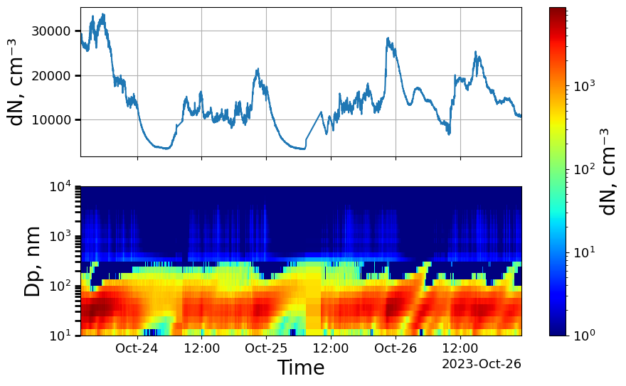
The resulting variable is an aerosol2d class object, with the same functionalities as the raw loaded data. It is thus possible to plot particle data in the broad size range from 10 nm (Nanoscan lower limit) to 10 µm (OPS upper limit).

The two datasets are combined by simply discarding the upper bins of the Nanoscan, while including all of the OPS bins, as the nanoscan is known to be uncertain at upper range of its particle size spectrum.

combined.plot_timeseries(y_3d=(1,0));
# as some bins have concentrations of 0 cm-3 it is necessary to set the lower limit to 1 via y_3d = (1,0)
# the upper limit of 0 indicates that the maximum value in the data should be used.