Dtypes, PM plots and exposure
This example demonstrates how to:
Load size-resolved ELPI data (
Aerosol2D)Inspect dtype, units, and particle density
Convert between different distribution types via
dtype_converterCompute cumulative Pₓ (e.g. PM₂.₅, PM₄.₂) with
PM_calcPlot PMₓ time series with
plot_pm_timeseriesAdjust assumed particle density with
set_densityUse
summarize_activitiesandsummarize_exposurefor PM-based metrics
[ ]:
import matplotlib.pyplot as plt
import aerosoltools as at
Load ELPI sample data
Initially load an ELPI test dataset.
[4]:
filename = r"..\..\tests\data\Sample_ELPI.txt"
elpi = at.Load_ELPI_file(filename)
################# Warning! #################
          Density ≠ 1.0 assumed
  Bin edges estimated via geometric means
###########################################
A warning is given, seeing that the density in the given raw data is not set equal to 1.0. The density of the raw data is read, loaded and stored within the generated elpi variable, but the user is still alerted.
Check dtype, unit, and density
The loader sets the initial distribution type (e.g. dN) and unit. Assumed particle density is stored in elpi.density (g/cm³).
[5]:
print("Initial dtype:", elpi.dtype)
print("Initial unit:", elpi.unit)
print("Initial density (g/cm³):", elpi.density)
Initial dtype: dN
Initial unit: cm⁻³
Initial density (g/cm³): 0.14
Change density and convert to mass distribution
We can update the assumed particle density with set_density() and then convert to a mass-based size distribution using dtype_converter("dM").
[7]:
# For illustration, set density to 1.5 g/cm³
elpi.set_density(1.5)
elpi.dtype_converter("dM")
print("Updated dtype:", elpi.dtype)
print("Updated density (g/cm³):", elpi.density)
print("Updated unit:", elpi.unit)
Updated dtype: dM
Updated density (g/cm³): 1.5
Updated unit: ug/m³
Compute PM fractions with PM_calc
We now calculate mass-based Pₓ metrics such as PM₂.₅ and PM₄.₂. The results are stored in elpi.extra_data as additional columns.
[8]:
# Compute cumulative PM2.5 and PM4.2 (µm cut points)
elpi.PM_calc(dtype="dM", PM=2.5)
elpi.PM_calc(dtype="dM", PM=4.2)
print([c for c in elpi.extra_data.columns if c.startswith("PM")])
['PM2.5', 'PM4.2']
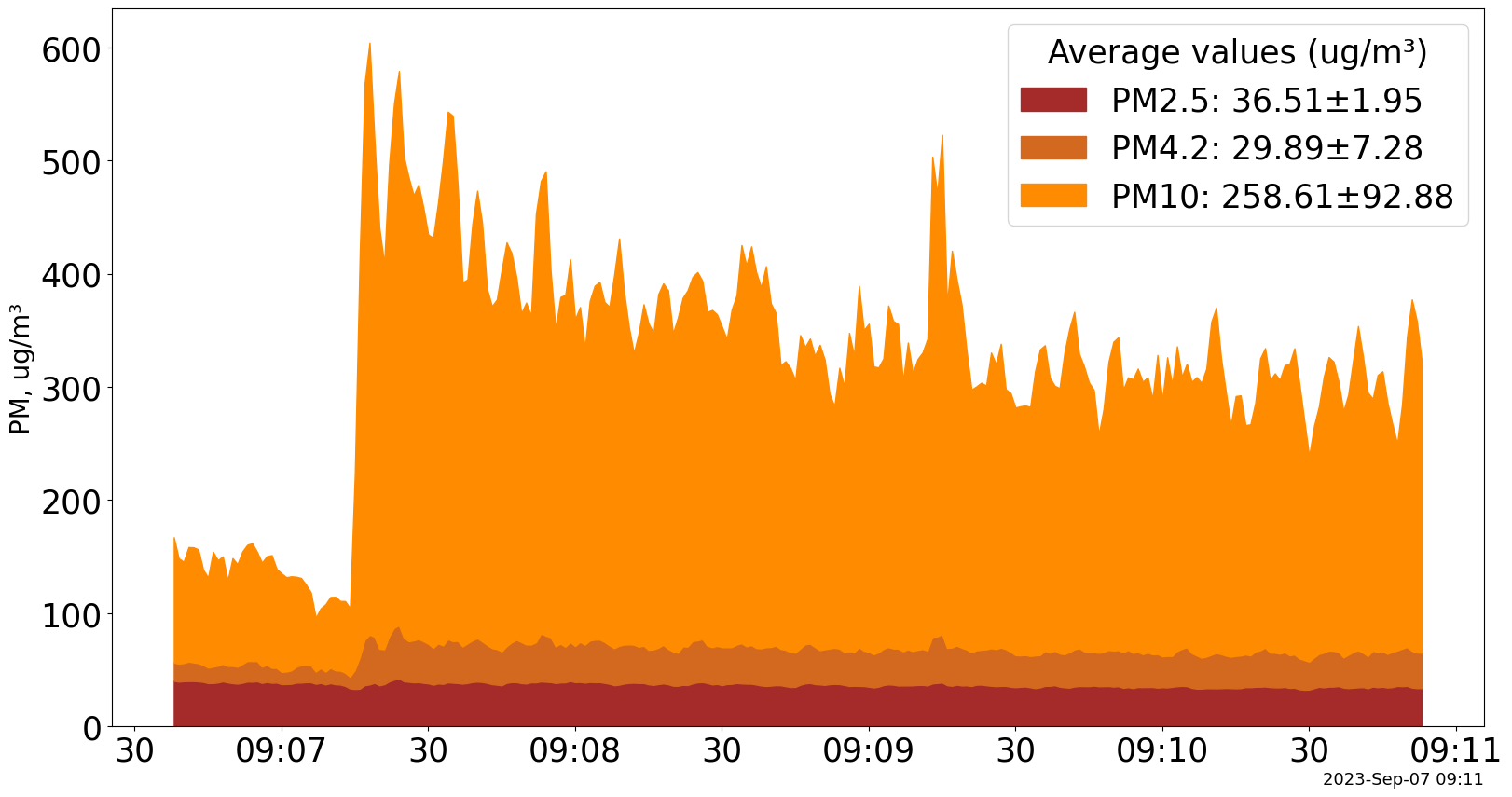
Plot PM time series
Use plot_pm_timeseries to visualize the evolution of PMₓ over time.
[12]:
elpi.plot_PM_timeseries(PM_values=[2.5, 4.2, 10])
[12]:
(<Figure size 1900x1000 with 1 Axes>, <Axes: ylabel='PM, ug/m³'>)
Define activities and summarize
As with Aerosol1D, we can mark time segments and compute activity-based statistics using summarize_activities().
[13]:
activity_periods = {
    "Background": [("2023/09/07 09:06:50", "2023/09/07 09:07:50")],
    "Emission":   [("2023/09/07 09:07:55", "2023/09/07 09:08:30")],
    "Decay":      [("2023/09/07 09:09:00", "2023/09/07 09:10:50")],
}
elpi.mark_activities(activity_periods)
summary = elpi.summarize_activities()
summary
Summary of aerosol properties (transposed):

+------------------------+----------+------------+----------+---------+
|                        | All data | Background | Emission |  Decay  |
+------------------------+----------+------------+----------+---------+
|    Duration (HH:MM)    |  00:04   |   00:01    |  00:00   |  00:01  |
|       PNC [cm⁻³]       |  197.44  |   222.84   |  203.63  | 179.39  |
|     PNC [cm⁻³] std     |   48.9   |   61.26    |  42.67   |  39.3   |
|      PM1 [µg/m³]       |  13.79   |   14.97    |  14.06   |  12.85  |
|    PM1 [µg/m³] std     |   1.15   |    0.89    |   0.26   |  0.38   |
|     PM2.5 [µg/m³]      |  36.51   |   37.94    |  37.83   |  34.95  |
|   PM2.5 [µg/m³] std    |   1.95   |    1.6     |   1.09   |  1.13   |
|      PM4 [µg/m³]       |  61.78   |   60.51    |  66.44   |  61.04  |
|    PM4 [µg/m³] std     |   6.28   |   10.08    |   2.77   |  3.12   |
|      PM10 [µg/m³]      |  325.0   |   320.29   |  374.75  | 318.69  |
|    PM10 [µg/m³] std    |  99.82   |   169.28   |  22.18   |  42.5   |
|   Total Mass [µg/m³]   | 1335.13  |  1421.95   | 1615.86  | 1225.18 |
| Total Mass [µg/m³] std |  549.75  |   896.41   |  216.46  | 248.88  |
|      Mode Dp [nm]      |  125.2   |   113.6    |  125.4   |  132.9  |
|    Mode Dp [nm] std    |  131.1   |   125.6    |  128.9   |  135.4  |
|     Median Dp [nm]     |  224.2   |   210.6    |  226.2   |  228.1  |
|   Median Dp [nm] std   |   68.6   |    76.9    |   66.2   |  67.3   |
|        GMD [nm]        |  203.3   |   193.0    |  201.4   |  212.6  |
|      GMD [nm] std      |   79.5   |    79.2    |   77.8   |  84.1   |
+------------------------+----------+------------+----------+---------+
[13]:
| Segment | Duration (HH:MM) | PNC [cm⁻³] | PNC [cm⁻³] std | PM1 [µg/m³] | PM1 [µg/m³] std | PM2.5 [µg/m³] | PM2.5 [µg/m³] std | PM4 [µg/m³] | PM4 [µg/m³] std | PM10 [µg/m³] | PM10 [µg/m³] std | Total Mass [µg/m³] | Total Mass [µg/m³] std | Mode Dp [nm] | Mode Dp [nm] std | Median Dp [nm] | Median Dp [nm] std | GMD [nm] | GMD [nm] std | |
|---|---|---|---|---|---|---|---|---|---|---|---|---|---|---|---|---|---|---|---|---|
| 0 | All data | 00:04 | 197.44 | 48.90 | 13.79 | 1.15 | 36.51 | 1.95 | 61.78 | 6.28 | 325.00 | 99.82 | 1335.13 | 549.75 | 125.2 | 131.1 | 224.2 | 68.6 | 203.3 | 79.5 |
| 1 | Background | 00:01 | 222.84 | 61.26 | 14.97 | 0.89 | 37.94 | 1.60 | 60.51 | 10.08 | 320.29 | 169.28 | 1421.95 | 896.41 | 113.6 | 125.6 | 210.6 | 76.9 | 193.0 | 79.2 |
| 2 | Emission | 00:00 | 203.63 | 42.67 | 14.06 | 0.26 | 37.83 | 1.09 | 66.44 | 2.77 | 374.75 | 22.18 | 1615.86 | 216.46 | 125.4 | 128.9 | 226.2 | 66.2 | 201.4 | 77.8 |
| 3 | Decay | 00:01 | 179.39 | 39.30 | 12.85 | 0.38 | 34.95 | 1.13 | 61.04 | 3.12 | 318.69 | 42.50 | 1225.18 | 248.88 | 132.9 | 135.4 | 228.1 | 67.3 | 212.6 | 84.1 |
Exposure summary for respirable dust (PM4.2)
Finally, we use summarize_exposure on the Aerosol2D object to obtain exposure metrics for PM₄.₂ during the Emission task, using Background as the background activity.
[15]:
exp = elpi.summarize_exposure(
    metric="PM4.2",
    activity="Emission",
    background="Background",  # use mean Background as background level
    exposure_hours=None,       # assume exposure equals task duration
    short_limit=1.0,
    long_limit=1.0,
    short_window="15min",
    twa_window="8h",
)
exp
Exposure summary for segment 'Emission' and metric 'PM4.2' (µg/m³):

+--------------------------------------------+----------+
|                   Metric                   | Emission |
+--------------------------------------------+----------+
|                   Metric                   |  PM4.2   |
|                    Unit                    |  µg/m³   |
|                Duration_min                |   0.6    |
|               Duration_HH:MM               |  00:00   |
|                    Mean                    |  71.797  |
|                    Std                     |  3.127   |
|                   Median                   |  71.21   |
|                    Max                     |  78.57   |
|                  Seg_TWA                   |  71.797  |
|                 Window_TWA                 |  64.657  |
|             Window_TWA_window              |    8h    |
|                Short_limit                 |   1.0    |
|                Short_window                |  15min   |
|         Short_limit_exceedance_min         |   0.6    |
|      Short_limit_exceedance_fraction       |   1.0    |
|   Short_limit_fullwindow_exceedance_min    |   0.02   |
| Short_limit_fullwindow_exceedance_episodes |    1     |
|                 Long_limit                 |   1.0    |
|            Long_limit_exceeded             |   True   |
|         Long_limit_exceedance_min          |   0.6    |
|                    C95                     |  76.709  |
|                    C99                     |  78.018  |
|                    IQR                     |  4.235   |
|                   Peaks                    |    0     |
+--------------------------------------------+----------+
[15]:
| Segment | Metric | Unit | Duration_min | Duration_HH:MM | Mean | Std | Median | Max | Seg_TWA | ... | Short_limit_exceedance_fraction | Short_limit_fullwindow_exceedance_min | Short_limit_fullwindow_exceedance_episodes | Long_limit | Long_limit_exceeded | Long_limit_exceedance_min | C95 | C99 | IQR | Peaks | |
|---|---|---|---|---|---|---|---|---|---|---|---|---|---|---|---|---|---|---|---|---|---|
| 0 | Emission | PM4.2 | µg/m³ | 0.6 | 00:00 | 71.797 | 3.127 | 71.21 | 78.57 | 71.797 | ... | 1.0 | 0.02 | 1 | 1.0 | True | 0.6 | 76.709 | 78.018 | 4.235 | 0 |
1 rows × 25 columns