2 — Time adjustments
Theme: getting a record onto the time base you need.
Instruments log on their own clocks and at their own intervals. These four operations — crop, shift, smooth and rebin — are what you use to line them up before comparing or combining anything.
Plots here are only used to show the effect of each step; the plotting API itself is covered in 5 — Plotting.
[1]:
import matplotlib.pyplot as plt

import aerosoltools as at

ops = at.load_data_from_folder(
    "../../tests/data/OPS_data", at.load_ops_file, search_word="OPS"
)
print(f"{len(ops.data)} rows, {ops.time[0]} -> {ops.time[-1]}")
/opt/hostedtoolcache/Python/3.11.15/x64/lib/python3.11/site-packages/tqdm/auto.py:21: TqdmWarning: IProgress not found. Please update jupyter and ipywidgets. See https://ipywidgets.readthedocs.io/en/stable/user_install.html
  from .autonotebook import tqdm as notebook_tqdm
Loading files: 100%|██████████| 4/4 [00:00<00:00, 113.28file/s]
File load summary:

+---------------+--------+--------+
|     File      | Status | Reason |
+---------------+--------+--------+
| OPS_data1.csv | Loaded |   -    |
| OPS_data2.csv | Loaded |   -    |
| OPS_data3.csv | Loaded |   -    |
| OPS_data4.csv | Loaded |   -    |
+---------------+--------+--------+
2223 rows, 2023-10-25 08:59:51 -> 2023-10-31 14:06:52
The record spans several days. Each operation below modifies the object in place by default; pass inplace=False to get a modified copy instead and leave the original alone.
Cropping
timecrop restricts the record to an interval. With focus=False it does the opposite and removes the interval.
[2]:
ops.timecrop(start="2023-10-25 08:00:00", end="2023-10-26 22:00:00")
print(f"{len(ops.data)} rows, {ops.time[0]} -> {ops.time[-1]}")
2079 rows, 2023-10-25 08:59:51 -> 2023-10-26 19:38:42
Shifting
timeshift moves every timestamp by a fixed offset — the usual fix when an instrument’s clock was set wrong, or was in another time zone.
[3]:
first_before = ops.time[0]
ops.timeshift(minutes=120)
print(f"{first_before}  ->  {ops.time[0]}")
2023-10-25 08:59:51 -> 2023-10-25 10:59:51
Smoothing
timesmooth applies a rolling window. It changes the values but not the number of samples or the timestamps.
[4]:
smoothed = ops.timesmooth(60, method="mean", inplace=False)
print(f"rows unchanged: {len(ops.data)} -> {len(smoothed.data)}")
rows unchanged: 2079 -> 2079
Rebinning
timerebin is the one that changes the time base: it resamples onto a regular grid, so the number of samples changes.
[5]:
rebinned = ops.timerebin("2.5h", inplace=False)
print(f"{len(ops.data)} rows -> {len(rebinned.data)} rows at 2.5 h")
2079 rows -> 15 rows at 2.5 h
Rebinning to a common frequency is how two instruments logging at different intervals are made comparable. Several functions do this for you when asked — plot_correlation and the calibration helpers take match="rebin" — but doing it explicitly is useful when you want the same grid everywhere.
The effect of each step
[6]:
source = at.load_data_from_folder(
    "../../tests/data/OPS_data", at.load_ops_file, search_word="OPS"
)

fig, axs = plt.subplots(nrows=2, ncols=2, figsize=(11, 6))

source.plot_total_conc(axs[0, 0])
axs[0, 0].set_title("As loaded")

step = source.copy_self()
step.timecrop(start="2023-10-25 08:00:00", end="2023-10-26 22:00:00")
step.plot_total_conc(axs[0, 1])
axs[0, 1].set_title("Cropped")

step.timesmooth(60, method="mean")
step.plot_total_conc(axs[1, 0])
axs[1, 0].set_title("Smoothed (60-sample window)")

step.timerebin("2.5h")
step.plot_total_conc(axs[1, 1])
axs[1, 1].set_title("Rebinned to 2.5 h")

plt.tight_layout()
Loading files: 100%|██████████| 4/4 [00:00<00:00, 126.15file/s]
File load summary:

+---------------+--------+--------+
|     File      | Status | Reason |
+---------------+--------+--------+
| OPS_data1.csv | Loaded |   -    |
| OPS_data2.csv | Loaded |   -    |
| OPS_data3.csv | Loaded |   -    |
| OPS_data4.csv | Loaded |   -    |
+---------------+--------+--------+
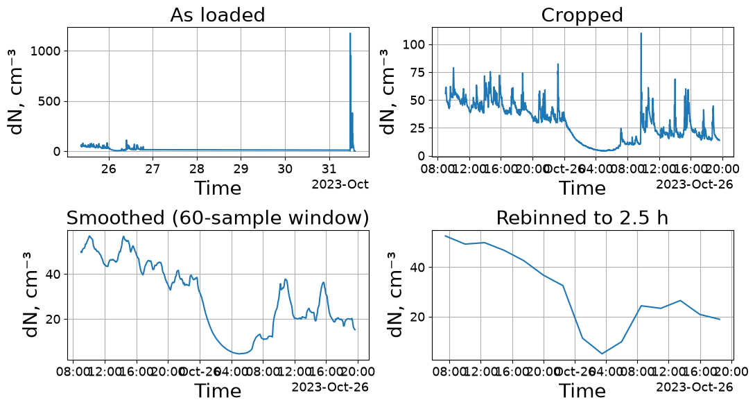
Smoothing flattens the peaks while keeping every sample; rebinning replaces the samples with far fewer, wider ones. Both reduce noise, but only rebinning changes what a “sample” means — which matters for any statistic computed afterwards.
Irregular sampling
Real records have gaps and jitter. Integrated quantities (time-weighted averages, exposure metrics) account for the actual spacing between samples rather than assuming a fixed interval, so an instrument that paused for ten minutes does not silently distort the result.
Next: 3 — Activities marks what was happening during a record.