13 — APS: dual size distributions
Theme: an instrument that sizes the same particle two different ways at once.
The TSI Aerodynamic Particle Sizer measures an aerodynamic diameter, from how a particle accelerates in a flow, and an optical diameter, from how much light it scatters. The two differ in a way that depends on particle shape and refractive index — so comparing them says something about what the particles are, not just how large they are.
An APS export therefore loads as Aerosol3d: two size distributions over time, plus the correlation between them.
[1]:
import matplotlib.pyplot as plt

import aerosoltools as at

aps = at.load_aps_file("../../tests/data/Sample_APS_correlated.txt")

print("type         :", type(aps).__name__)
print("is_correlated:", aps.is_correlated)
type         : Aerosol3d
is_correlated: True
/opt/hostedtoolcache/Python/3.11.15/x64/lib/python3.11/site-packages/tqdm/auto.py:21: TqdmWarning: IProgress not found. Please update jupyter and ipywidgets. See https://ipywidgets.readthedocs.io/en/stable/user_install.html
  from .autonotebook import tqdm as notebook_tqdm
is_correlated distinguishes the two kinds of export. A correlated file carries both axes and the joint distribution; an aerodynamic-only file loads as a plain Aerosol2D, because there is no second axis to pair with.
[2]:
aero_only = at.load_aps_file("../../tests/data/Sample_APS_aero.txt")
print("aerodynamic-only export loads as:", type(aero_only).__name__)
aerodynamic-only export loads as: Aerosol2D
The two axes
Each axis is available as an ordinary size-resolved dataset, so everything from the earlier notebooks works on it. Note that they do not share a bin structure: the two sizing principles have different resolutions and cover different ranges.
[3]:
print(f"aerodynamic: {len(aps.aerodynamic.bin_mids):2d} bins, "
      f"{aps.aerodynamic.bin_mids.min():7.1f} - {aps.aerodynamic.bin_mids.max():8.1f} nm")
print(f"optical    : {len(aps.optical.bin_mids):2d} bins, "
      f"{aps.optical.bin_mids.min():7.1f} - {aps.optical.bin_mids.max():8.1f} nm")
aerodynamic: 52 bins,   514.5 -  19810.0 nm
optical    : 16 bins,   561.1 -  17822.4 nm
Comparing the two distributions
Drawing both on one axes needs a colour per dataset. plot_psd normally colours by activity, so two datasets would otherwise come out the same colour and read as a single line doubling back on itself. Pass color and label to name the dataset instead.
The shaded band around each curve is ±1 standard deviation across time, not an uncertainty on the mean.
[4]:
fig, ax = plt.subplots(figsize=(8, 5))

aps.aerodynamic.plot_psd(ax=ax, activities=["All data"],
                         color="tab:blue", label="aerodynamic")
aps.optical.plot_psd(ax=ax, activities=["All data"],
                     color="tab:orange", label="optical")

ax.set_xscale("log")
ax.set_title("The same particles, sized two ways")
ax.legend(loc="upper right")
plt.tight_layout()
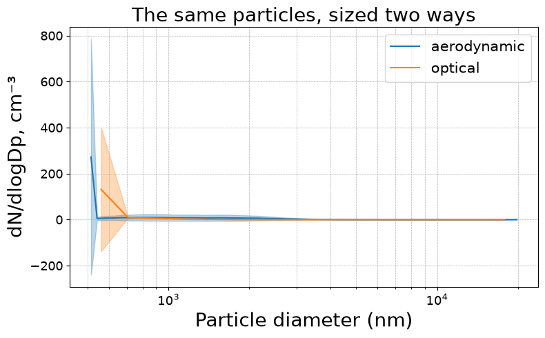
The separation between the curves is the physical signal. For spherical particles of known refractive index the two sizings agree; they diverge as particles become irregular, porous, or optically unusual. The optical distribution here is both coarser and narrower, which is what a small number of wide bins produces.
Working with one axis
as_2d returns an independent copy of one axis — modify it freely without touching the parent.
[5]:
standalone = aps.as_2d("aerodynamic")
print(type(standalone).__name__, "with", len(standalone.bin_mids), "bins")
Aerosol2D with 52 bins
axis_view returns a live view instead, with activities kept in sync with the parent. Use axis_view when you want marked activities to follow, and as_2d when you want an independent object.
[6]:
view = aps.axis_view("optical")
print(type(view).__name__, "- activities stay synced with the parent")
Aerosol2D - activities stay synced with the parent
The instrument’s own comparison
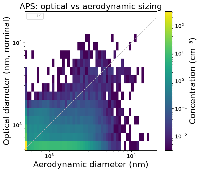
plot_aero_vs_optical shows the relationship between the two diameters directly, rather than as two separate distributions.
[7]:
fig, ax = aps.plot_aero_vs_optical()
The joint distribution
For each time step the instrument records how many particles fell in each (aerodynamic, optical) pair of bins. correlation_cube returns that as a dense time × optical × aerodynamic array.
[8]:
cube = aps.correlation_cube()
print("type:", type(cube).__name__)
type: CorrelationCube
[9]:
fig, ax = aps.plot_aero_optical_3d()
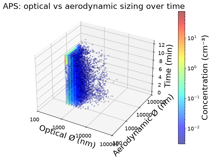
This is what makes an APS more than two instruments in a box: it records which optical size each aerodynamically-sized particle had, rather than giving two independent histograms that happen to cover the same air.
Summaries
Because each axis is a normal size-resolved dataset, mass fractions, statistics and exposure metrics all work per axis.
[10]:
aps.aerodynamic.summarize_activities(metrics=["PNC"], stats=["mean", "median", "max"])
Summary of aerosol properties (transposed):

+-------------------+----------+
|                   | All data |
+-------------------+----------+
| Duration (HH:MM)  |  00:12   |
|    PNC [cm⁻³]     |  15.19   |
| PNC [cm⁻³] median |   3.02   |
|  PNC [cm⁻³] max   |  117.71  |
+-------------------+----------+
[10]:
| Segment | Duration (HH:MM) | PNC [cm⁻³] | PNC [cm⁻³] median | PNC [cm⁻³] max | |
|---|---|---|---|---|---|
| 0 | All data | 00:12 | 15.19 | 3.02 | 117.71 |
Next: 15 — ACSM.