2D heatmap
The whole size distribution over time, as a colour map: time across, particle diameter up, concentration as colour. The quickest way to see which sizes an event produced, rather than just how much.
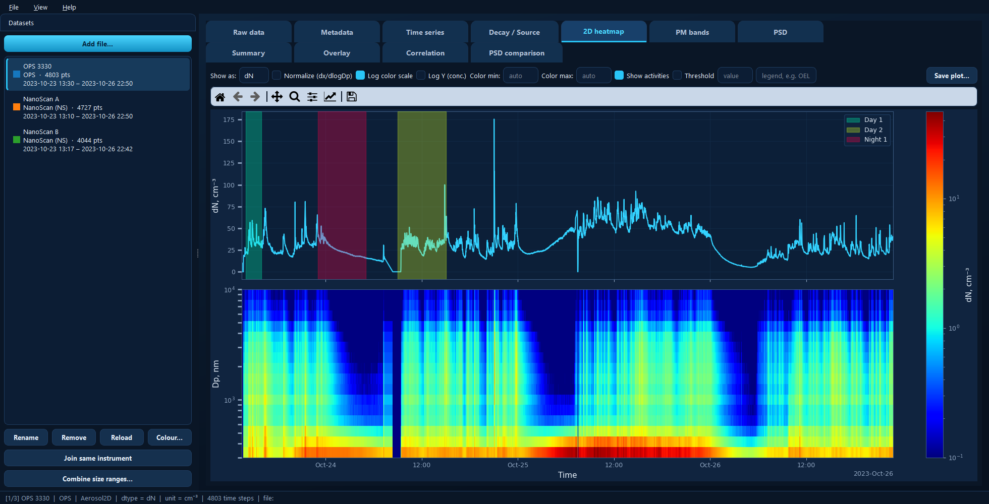
Total concentration on top, the time–size distribution below. Reading up a column tells you the size distribution at that moment.
Available for: size-resolved (2D) datasets only — the tab is absent for single-channel instruments.
The two panels
The top panel is total concentration over time — the same trace as the Time series tab, for orientation.
The bottom panel is the heatmap. Each column is one timestamp’s size distribution. A rise that appears only in the lowest rows is a fresh, fine-particle source; one spread across the upper rows points at coarser dust.
Both panels share a time axis, so zooming one zooms the other.
Show as
The distribution basis for display only — number (dN), mass (dM), surface
area (dS) or volume (dV). The dataset itself stays as number.
This changes the picture more than you might expect: a number distribution is dominated by the smallest particles, a mass distribution by the largest. Mass, surface and volume all depend on the particle density set on the Metadata tab.
Normalize (dx/dlogDp)
Divides each bin by its width in log-diameter space. Size bins are not equally wide, so without this a wide bin looks more concentrated simply because it collects more particles. Leave it on to compare bins fairly; turn it off to read the raw per-bin concentration.
Colour scale
Log color scale spreads several decades of concentration across the colours at once, which is normally what you want — aerosol concentrations vary by orders of magnitude, and a linear scale tends to show one bright band and nothing else. It needs positive values, so zeros are floored.
Color min and Color max pin the scale to fixed limits; leave blank for automatic. Fixing them is how you make two datasets comparable — otherwise each one auto-scales to itself and the colours mean different things.
Other controls
Log Y (conc.) log-scales the y-axis of the top total-concentration panel.
Show activities shades the marked periods on the top panel.
Under the hood
This is the two-panel figure plot_timeseries produces for size-resolved data:
import aerosoltools as at

data = at.load_ops_file("measurement.csv")
data.plot_timeseries(log=True, mark_activities=True, dtype="dN")
See 5 — Plotting.