PM bands
Splits the size distribution into size-selective fractions — PM₁₀, PM₂.₅, PM₀.₅ and the bands between them — and stacks them over time. This is the view that maps onto how exposure limits are usually written.
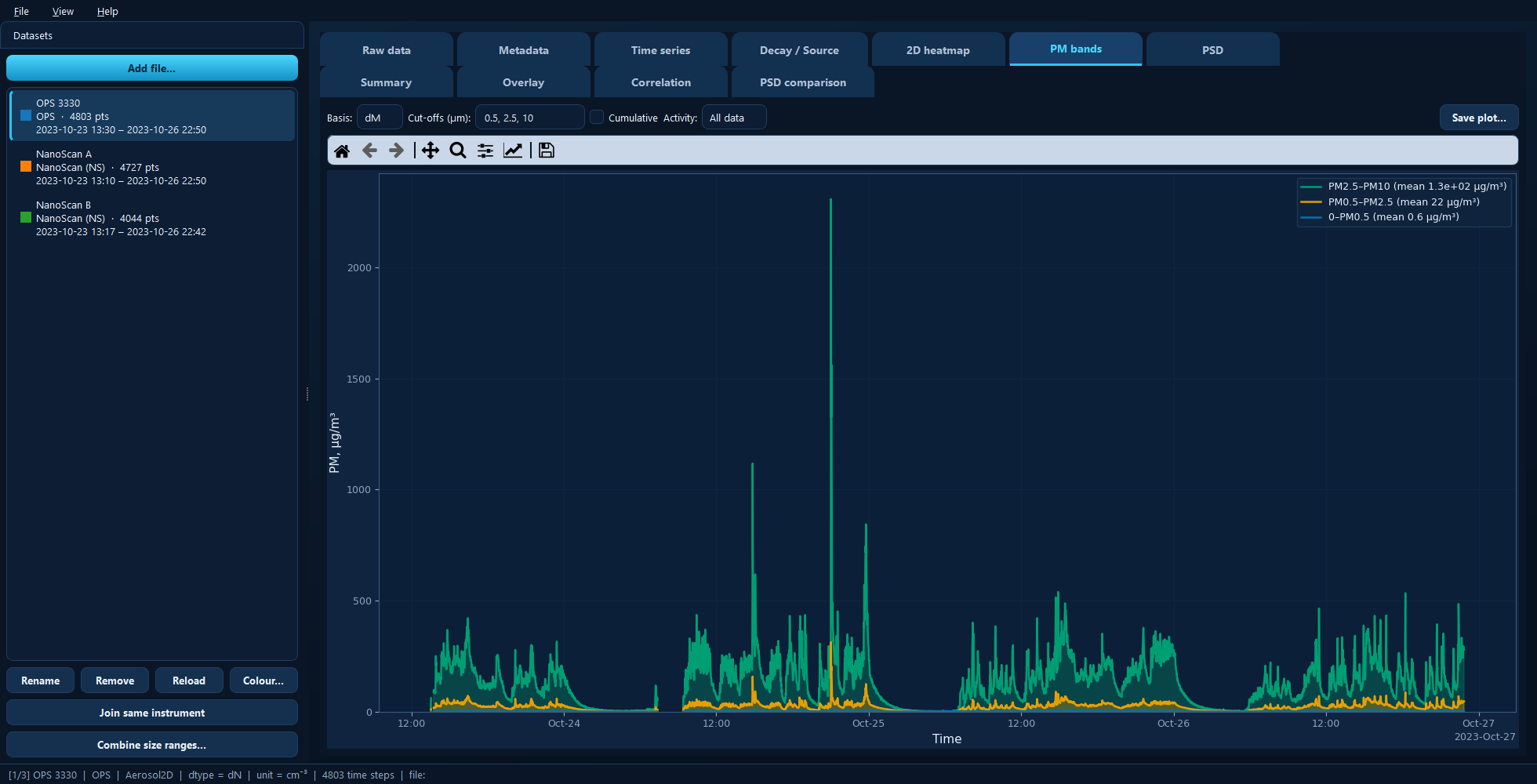
Three stacked bands with their mean concentrations in the legend. The band heights add up to the total below the largest cut-off.
Available for: size-resolved (2D) datasets only.
Cut-offs
A comma-separated list of cut diameters in micrometres — 0.5, 2.5, 10 by
default. Each cut-off defines a size-selective fraction: PM₂.₅ is everything
below 2.5 µm.
You can use any cut-offs the instrument’s size range supports. Asking for a cut-off beyond the largest bin simply gives you everything the instrument measured.
Basis
The quantity the fractions are computed on: mass (dM, the default and the usual
choice for PM), number (dN), surface area (dS) or volume (dV).
PM limits are written in mass, so dM is normally what you want — and it depends
on the particle density set on the Metadata tab. Number-based
bands are useful for a different question: whether an event was many small
particles or a few large ones.
Cumulative
Changes what each band means:
Off (default) — each band is the fraction between successive cut-offs:
0–PM0.5,PM0.5–PM2.5,PM2.5–PM10. The bands are independent and stack to the total.On — each band is everything below its cut-off: PM₀.₅, PM₂.₅, PM₁₀. The bands overlap, each containing the ones below it.
Use the independent bands to see which size range an event lives in; use cumulative when you want the PM values as an exposure limit defines them.
Activity
Restricts the plot to one marked activity. Leave it on All data for the whole record.
The legend reports each band’s mean over whatever is shown, so switching activity gives you the per-task means directly.
Under the hood
import aerosoltools as at

data = at.load_ops_file("measurement.csv")
data.plot_PM_timeseries(
    PM_values=[0.5, 2.5, 10],   # Cut-offs (µm)
    dtype="dM",                 # Basis
    cumulative=False,           # Cumulative
    activity="All data",        # Activity
)
See 5 — Plotting and 4 — Statistics and exposure.