5 — Plotting
Theme: the built-in plots and the arguments that control them.
Four plotting methods cover most needs. Every one returns the Matplotlib figure and axes, so anything not offered as an argument can still be done afterwards with ordinary Matplotlib.
Specialised plots live with their topics: 8 — PSD fitting, 10a — Correlation and agreement and 13 — APS.
[1]:
import matplotlib.pyplot as plt

import aerosoltools as at

elpi = at.load_elpi_file("../../tests/data/Sample_ELPI.txt")
elpi.mark_activities({
    "Background": [("2023-09-07 09:06:50", "2023-09-07 09:07:50")],
    "Emission":   [("2023-09-07 09:07:55", "2023-09-07 09:08:30")],
    "Decay":      [("2023-09-07 09:09:00", "2023-09-07 09:10:50")],
})
/opt/hostedtoolcache/Python/3.11.15/x64/lib/python3.11/site-packages/tqdm/auto.py:21: TqdmWarning: IProgress not found. Please update jupyter and ipywidgets. See https://ipywidgets.readthedocs.io/en/stable/user_install.html
  from .autonotebook import tqdm as notebook_tqdm
/home/runner/work/aerosoltools/aerosoltools/src/aerosoltools/loaders/elpi.py:525: RuntimeWarning: ELPI density is not 1.0 g/cm3; bin edges were estimated from geometric means of CalculatedDi values.
  return load_elpi_file_txt(
Total concentration over time
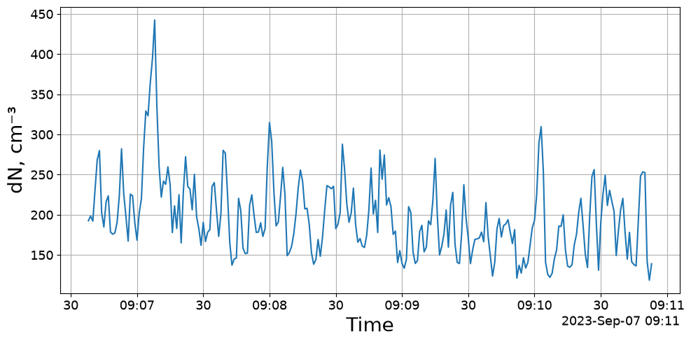
plot_total_conc is the simplest view: one line, whatever the instrument’s primary measurement is. It works on every class.
[2]:
fig, ax = elpi.plot_total_conc()
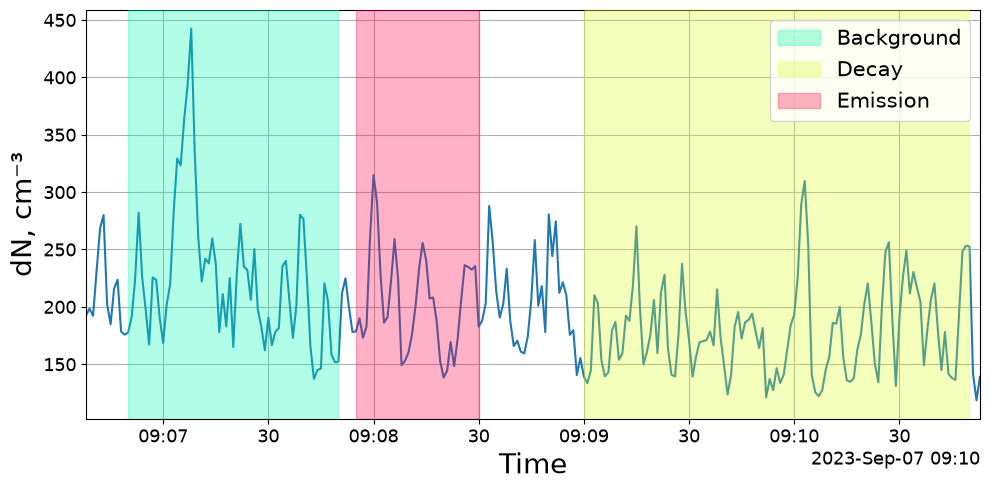
mark_activities=True shades the marked periods, which is usually what makes a time series readable.
[3]:
fig, ax = elpi.plot_total_conc(mark_activities=True)
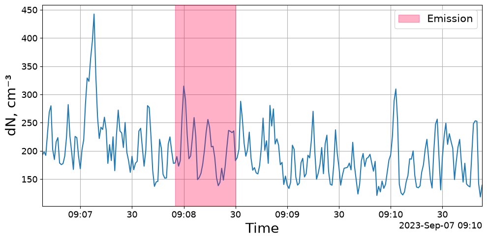
Pass a list instead of True to shade only some activities.
[4]:
fig, ax = elpi.plot_total_conc(mark_activities=["Emission"])
Size-resolved time series
For size-resolved data plot_timeseries adds a heat map of the size distribution below the total concentration.
[5]:
fig, axs = elpi.plot_timeseries()
========================================================================
WARNING (plot_timeseries):
  PSD data contain zero or negative values, or the lower
  color-scale limit is ≤ 0. Falling back to *linear*
  color scale for the concentration heatmap.

  To enforce log-scaled concentration, set y_3d to use a
  strictly positive lower limit, for example:
      y_3d = (1, 0)
  which clips values below 1 and allows log scaling.
========================================================================
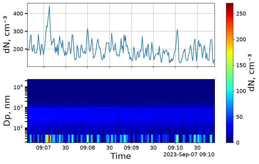
Two arguments control the axes:
y_tot— limits for the total-concentration panely_3d— colour limits for the heat map
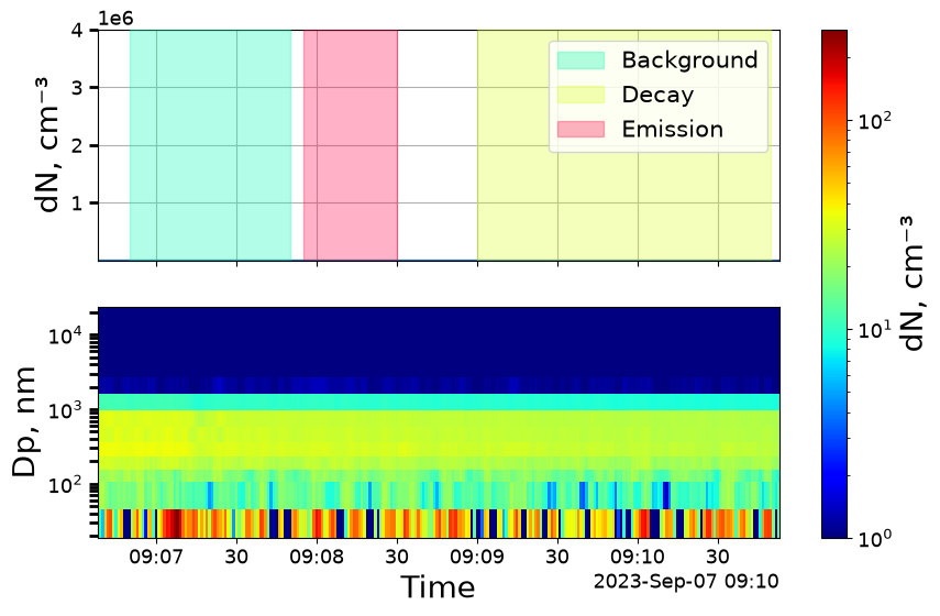
In both, 0 means “use the data”. The lower bound on y_3d matters: the colour scale is logarithmic by default, and bins reading exactly zero cannot be shown on a log scale, so setting a floor of 1 avoids a mostly empty plot.
[6]:
fig, axs = elpi.plot_timeseries(y_3d=(1, 0), y_tot=(0, 4e6), mark_activities=True)
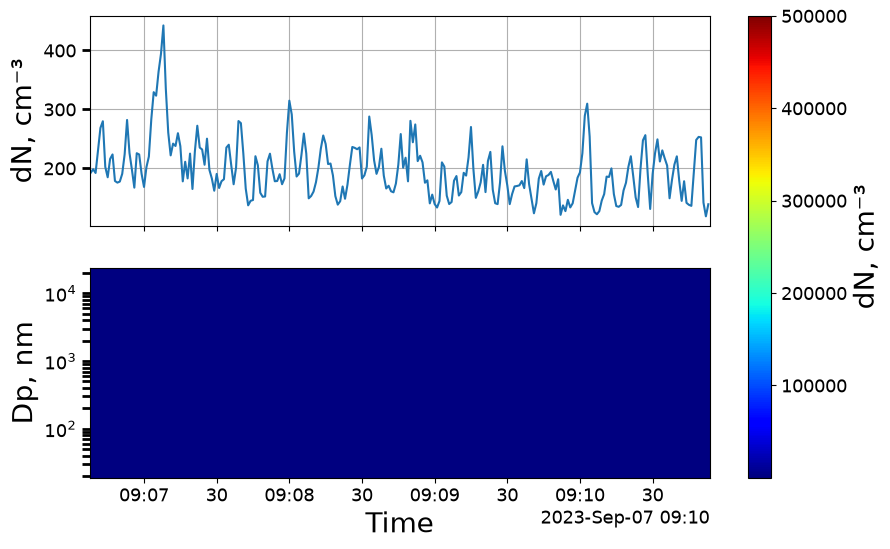
log=False switches the heat map to a linear colour scale.
[7]:
fig, axs = elpi.plot_timeseries(y_3d=(1, 5e5), log=False)
Size distributions
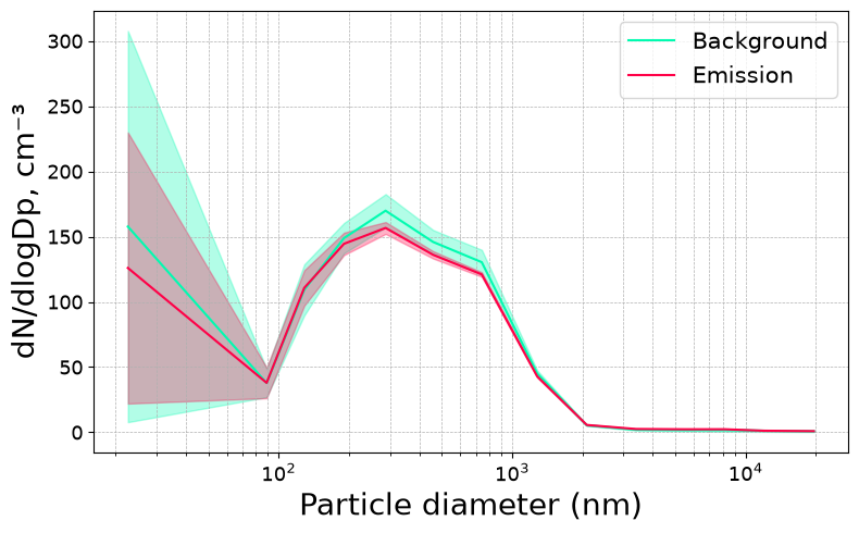
plot_psd draws the average size distribution. With activities marked it draws one curve per activity, which is the quickest way to see how a process changed the distribution.
[8]:
fig, ax = elpi.plot_psd()
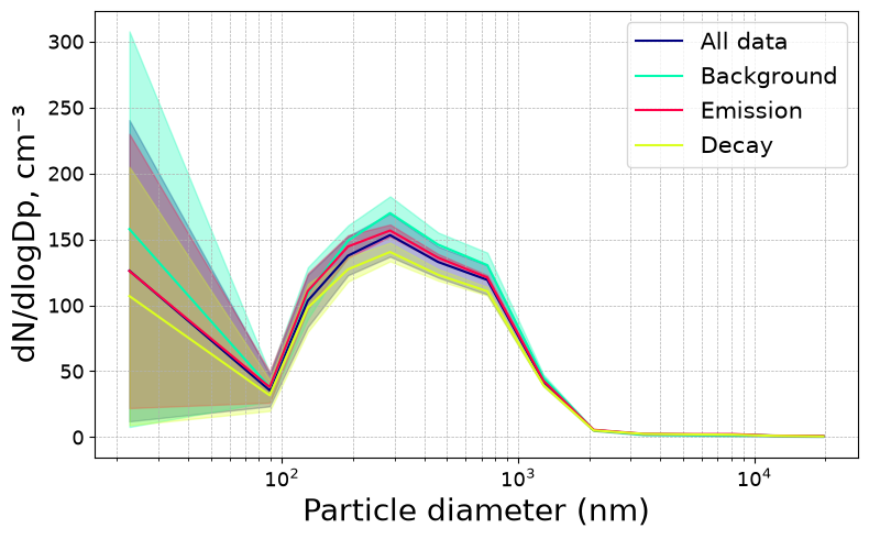
activities selects which curves to draw.
[9]:
fig, ax = elpi.plot_psd(activities=["Background", "Emission"])
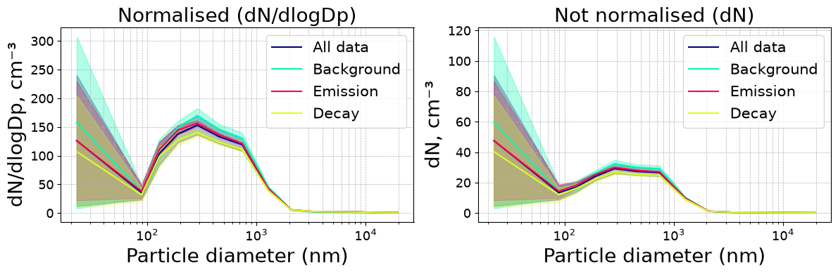
normalize controls dlogDp normalisation. Normalised distributions (dN/dlogDp, the default) are comparable between instruments with different bin widths; unnormalised ones show the raw per-bin concentration.
[10]:
fig, axs = plt.subplots(ncols=2, figsize=(12, 4))
elpi.plot_psd(normalize=True, ax=axs[0])
axs[0].set_title("Normalised (dN/dlogDp)")
elpi.plot_psd(normalize=False, ax=axs[1])
axs[1].set_title("Not normalised (dN)")
plt.tight_layout()
PM fractions over time
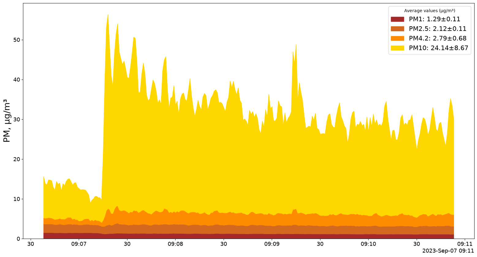
plot_PM_timeseries draws cumulative mass fractions. PM_values chooses the cut diameters, in µm.
[11]:
fig, ax = elpi.plot_PM_timeseries(PM_values=[1, 2.5, 4.2, 10])
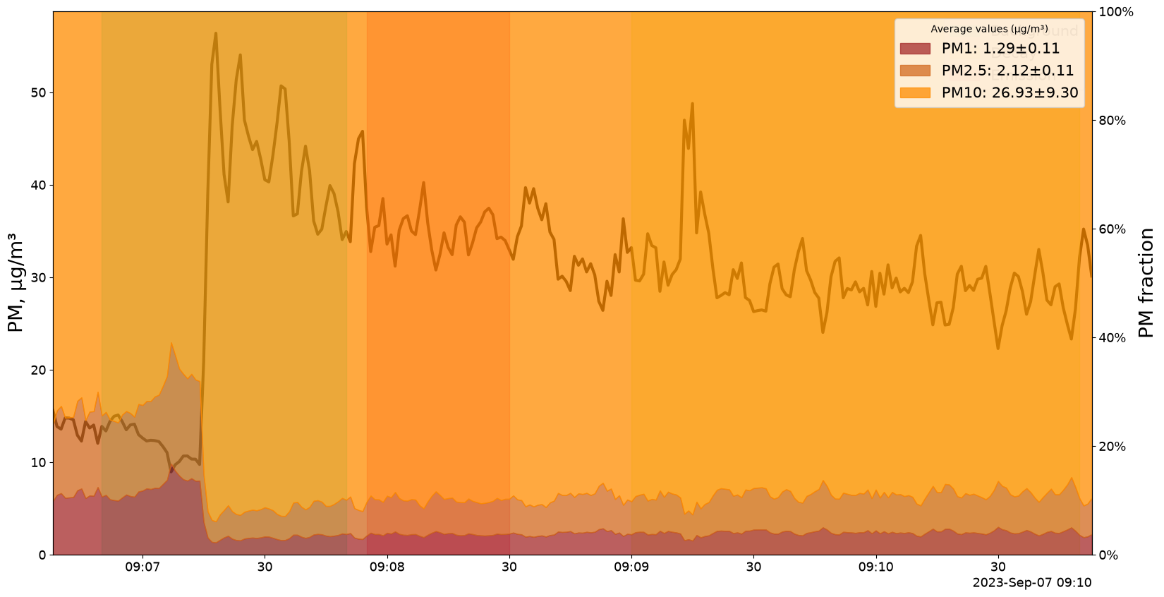
fraction=True plots each cut as a share of the total rather than an absolute concentration — useful for seeing a shift between coarse and fine particles that an absolute plot hides.
[12]:
fig, ax = elpi.plot_PM_timeseries(PM_values=[1, 2.5, 10], fraction=True,
                                  mark_activities=True)
Supplying your own axes
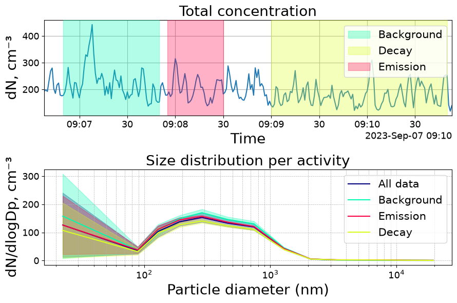
Every method takes an axes argument (ax, or ax1/ax2 for the two-panel time series), so plots can be composed into a figure you control.
[13]:
fig, axs = plt.subplots(nrows=2, figsize=(9, 6))

elpi.plot_total_conc(axs[0], mark_activities=True)
axs[0].set_title("Total concentration")

elpi.plot_psd(ax=axs[1])
axs[1].set_title("Size distribution per activity")

plt.tight_layout()
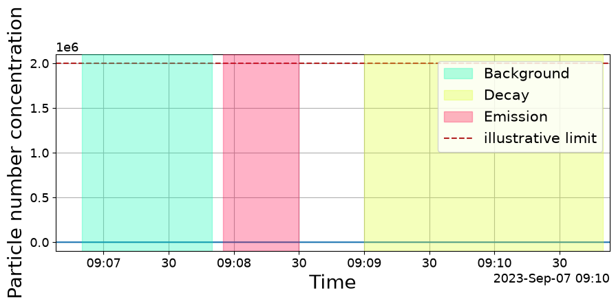
Because the figure and axes are returned, the result is an ordinary Matplotlib figure — restyle, annotate or save it however you normally would.
[14]:
fig, ax = elpi.plot_total_conc(mark_activities=True)
ax.set_ylabel("Particle number concentration")
ax.axhline(2e6, linestyle="--", color="firebrick", label="illustrative limit")
ax.legend(loc="upper right")
fig.set_size_inches(9, 3.5)