8 — PSD fitting
Theme: describing a measured size distribution as a small number of lognormal modes.
A distribution with 30-odd bins is hard to compare or report. Fitting it as one or more lognormal modes reduces it to a few numbers with physical meaning: a geometric mean diameter, a width, and a magnitude per mode.
[1]:
import numpy as np

import aerosoltools as at

smps = at.load_smps_file("../../tests/data/Sample_SMPS.txt")
fig, ax = smps.plot_psd()
/opt/hostedtoolcache/Python/3.11.15/x64/lib/python3.11/site-packages/tqdm/auto.py:21: TqdmWarning: IProgress not found. Please update jupyter and ipywidgets. See https://ipywidgets.readthedocs.io/en/stable/user_install.html
  from .autonotebook import tqdm as notebook_tqdm
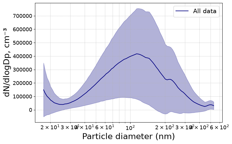
Fitting a single mode
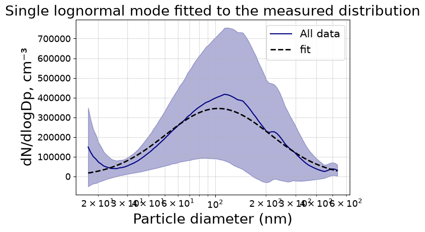
fit_psd takes an initial guess per mode: mu (geometric mean diameter, nm), sigma (geometric standard deviation, dimensionless, > 1) and factor (the magnitude). Lists of length n fit n modes.
[2]:
fit = smps.fit_psd(mu=[80], sigma=[1.8], factor=[1e4])
fit.modes
[2]:
{'mu': array([104.02098831]),
 'sigma': array([2.06998409]),
 'factor': array([273214.91995989])}
The result carries the fitted parameters and their uncertainties.
[3]:
for i in range(len(fit.modes["mu"])):
    print(f"mode {i + 1}")
    print(f"  mu     = {fit.modes['mu'][i]:8.2f} +/- {fit.errors['mu'][i]:.2f} nm")
    print(f"  sigma  = {fit.modes['sigma'][i]:8.3f} +/- {fit.errors['sigma'][i]:.3f}")
    print(f"  factor = {fit.modes['factor'][i]:8.1f} +/- {fit.errors['factor'][i]:.1f}")
mode 1
  mu     =   104.02 +/- 2.15 nm
  sigma  =    2.070 +/- 0.033
  factor = 273214.9 +/- 9807.9
PSDFitResult is a NamedTuple, so it also unpacks as a plain tuple if you prefer.
[4]:
modes, errors = fit
list(modes)
[4]:
['mu', 'sigma', 'factor']
Drawing the fit
evaluate returns the fitted curve at any diameters — the total first, then each mode separately.
[5]:
import matplotlib.pyplot as plt

dp = np.logspace(np.log10(smps.bin_mids.min()), np.log10(smps.bin_mids.max()), 200)
total, per_mode = fit.evaluate(dp)

fig, ax = plt.subplots(figsize=(7, 4.5))
smps.plot_psd(ax=ax, activities=["All data"])
ax.plot(dp, total, "k--", lw=2, label="fit")
ax.set_xscale("log")
ax.legend()
ax.set_title("Single lognormal mode fitted to the measured distribution")
[5]:
Text(0.5, 1.0, 'Single lognormal mode fitted to the measured distribution')
Fitting several modes
Real aerosols are often bimodal — a fresh nucleation mode plus an aged accumulation mode. Give one starting guess per mode.
[6]:
two = smps.fit_psd(mu=[30, 120], sigma=[1.6, 1.9], factor=[5e3, 1e4])

for i in range(len(two.modes["mu"])):
    print(f"mode {i + 1}: mu = {two.modes['mu'][i]:7.2f} nm, "
          f"sigma = {two.modes['sigma'][i]:.3f}, "
          f"factor = {two.modes['factor'][i]:9.1f}")
mode 1: mu =   56.24 nm, sigma = 5.000, factor =  100431.0
mode 2: mu =  112.98 nm, sigma = 1.695, factor =  218001.3
[7]:
total2, per_mode2 = two.evaluate(dp)

fig, ax = plt.subplots(figsize=(7, 4.5))
smps.plot_psd(ax=ax, activities=["All data"])
ax.plot(dp, total2, "k--", lw=2, label="fit (2 modes)")
for i, mode in enumerate(per_mode2):
    ax.plot(dp, mode, ":", lw=1.5, label=f"mode {i + 1}")
ax.set_xscale("log")
ax.legend()
[7]:
<matplotlib.legend.Legend at 0x7f64c2860a90>
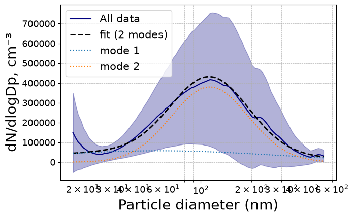
The starting guess matters. A fit is a local optimisation, so guesses far from the truth can converge somewhere unhelpful — start from where you can see modes in the plot.
Fitting one activity
period restricts the fit to a marked activity, which is how you compare the distribution during a process against the background.
[8]:
smps.mark_activities({
    "Emission":   [("2018-02-27 10:18:00", "2018-02-27 11:30:00")],
    "Background": [("2018-02-27 13:48:00", "2018-02-27 14:39:00")],
})

for activity in ["Emission", "Background"]:
    result = smps.fit_psd(period=activity, mu=[80], sigma=[1.8], factor=[1e4])
    print(f"{activity:11s} mu = {result.modes['mu'][0]:7.2f} nm, "
          f"sigma = {result.modes['sigma'][0]:.3f}")
Emission    mu =  109.51 nm, sigma = 2.191
Background  mu =   87.92 nm, sigma = 1.942
Evaluating a distribution without fitting
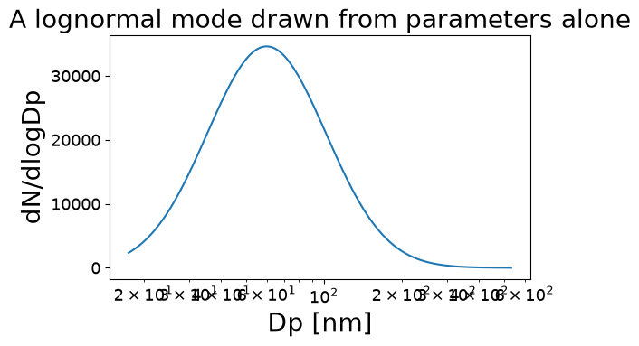
lognormal_modes is the underlying model, exposed directly. It takes (mu, sigma, factor) triples — one per mode — and returns the total and the individual modes, the same shape evaluate gives. Use it to draw a distribution from parameters you already have: from a fit, from the literature, or to sanity-check a starting guess before fitting.
[9]:
guess, _ = at.lognormal_modes(dp, [(60, 1.7, 2e4)])

fig, ax = plt.subplots(figsize=(6, 3.5))
ax.plot(dp, guess)
ax.set_xscale("log")
ax.set_xlabel("Dp [nm]")
ax.set_ylabel("dN/dlogDp")
ax.set_title("A lognormal mode drawn from parameters alone")
[9]:
Text(0.5, 1.0, 'A lognormal mode drawn from parameters alone')
Rebuilding the fitted curve from the modes a fit returned is the same call:
[10]:
triples = list(zip(two.modes["mu"], two.modes["sigma"], two.modes["factor"]))
rebuilt, _ = at.lognormal_modes(dp, triples)

print("matches evaluate():", bool((abs(rebuilt - total2) < 1e-9).all()))
matches evaluate(): True
Next: 9 — Decay and source fitting.