Aero ↔ Optical
Shows an APS’s two size measurements against each other: for a chosen moment, how much of the aerosol sat in each combination of optical and aerodynamic diameter. The relationship between the two is a property of the particles — their shape and density — so this view says something about what you measured, not just how much.
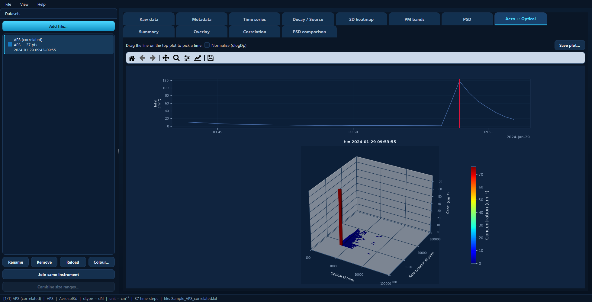
The time cursor (red) parked on a peak, and the correlated optical × aerodynamic distribution at that instant below.
Available for: a correlated APS only — an
Aerosol3d that carries both size axes. Every other
dataset, including an APS without the correlated output, has no such tab.
If you only need one of the two axes, the Metadata tab’s Show axis (APS) setting picks which one the ordinary 2D tabs (heatmap, PM bands, PSD) work on.
The two panels
The top panel is total concentration over time, carrying a red time cursor. Drag it to choose the moment shown below; the timestamp is printed above the lower panel.
The bottom panel is a 3-D bar plot of the correlated distribution at that moment. One bar per (optical, aerodynamic) size-bin pair, with both its height and its colour showing concentration — so it reads like a surface while keeping the unequally sized bins visibly separate.
The colour scale is fixed to the dataset’s global range, not rescaled per timestamp. That is deliberate: it means dragging the cursor through time gives a fair comparison, and a bar that grows really is growing.
Reading it
Bars along the diagonal are particles whose optical and aerodynamic diameters agree — roughly spherical, with a density near the calibration assumption. Bars off the diagonal are the interesting ones: an aerodynamic diameter well above the optical one points to dense particles, and the reverse suggests low-density or irregular, chain-like agglomerates.
Normalize (dlogDp)
Divides each cell by both log bin widths — dN/(dlogDp_optical · dlogDp_aerodynamic) — so bins of unequal width are comparable. Without it, a wide bin looks more concentrated simply because it spans more diameters.
The top total-concentration panel always stays on the raw counts.
Under the hood
A correlated APS loads as Aerosol3d, which holds both
distributions and can hand out either axis as an ordinary 2D object:
import aerosoltools as at

data = at.load_aps_file("Sample_APS_correlated.txt")
data.is_correlated                  # True for this file
aero = data.axis_view("aerodynamic")   # the Show axis (APS) setting
opt = data.axis_view("optical")
See 13 — APS.