Metadata
What the program knows about the dataset, plus the instrument-specific settings that belong to it: particle density, size-bin cropping, diffusion-loss correction and calibration. If a number looks wrong elsewhere in the app, this is usually where you fix it.
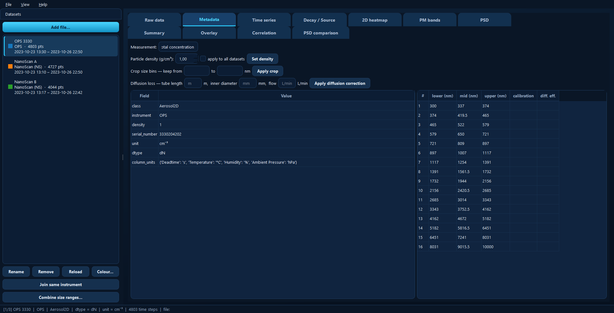
Metadata extracted from the file, the full size-bin table, and the controls that belong to the dataset itself.
Available for: every dataset. The size-bin table and the size-related controls appear only for size-resolved data.
The metadata table
Read-only. Shows what the loader extracted from the raw file and what the program has maintained since — instrument, serial number, units, sampling settings and any loader-specific fields. Worth checking after loading an unfamiliar file.
The size-bin table
Every size bin’s edges and midpoint diameter. When you apply a calibration or a diffusion-loss correction, this table also shows each bin’s calibration function and transmission efficiency, so you can see exactly what was applied per bin.
Measurement
The name of the measured quantity — Cl₂, IR BCc, and so on. It replaces the
generic “Total concentration” on the y-axis and in legends across every pane.
Clear the field to go back to the default label.
Mostly relevant for gas and black-carbon instruments, where “concentration” alone is ambiguous.
Particle density
The density (g/cm³) used for every mass-based conversion — dM in the plots and
exports, and the PM bands. The default comes from the file where the instrument
records it, otherwise from a sensible assumption; set it to the density of the
material you actually measured.
Tick apply to all datasets to push the same value to every dataset in the project at once, which is normally what you want when several instruments sampled the same aerosol.
For an ELPI, density does more than scale mass: the instrument’s size bins are themselves density-dependent, so changing it recomputes the particle sizes.
Show axis (APS)
Only for a correlated APS. Chooses which of its two size axes — Aerodynamic or Optical — the other tabs show and analyse. Both behave as ordinary size-resolved data. The Aero ↔ Optical tab shows the two together.
Crop size bins
Drops the bins outside the range you give, in nanometres. Useful when an instrument’s first or last bins are unreliable — a common case, and one worth checking on the PSD tab, where a bad edge bin distorts a fit.
This is a structural change: it alters the dataset. Use Reload in the sidebar to undo it.
Diffusion loss correction
Corrects for particles lost to the walls of the sampling tube, which matters most for the smallest sizes and long or narrow tubing. Enter the tube length (m), inner diameter (mm) and flow (L/min), then click Apply diffusion correction: each size bin is divided by its transmission efficiency to recover the concentration upstream of the tube. The per-bin efficiencies then appear in the size table.
Also structural — Reload undoes it.
Calibration
Shows a calibration fitted for this instrument on the Correlation tab.
Apply calibration toggles it on and off. With it off, every pane shows the original, uncalibrated data.
Reset removes the calibration entirely and restores the original data.
Under the hood
import aerosoltools as at

data = at.load_ops_file("measurement.csv")
data.set_density(2.5)                          # Particle density
data.correct_diffusion_losses(                 # Diffusion loss correction
    D_tube=0.004,   # inner diameter, m
    L=1.5,          # tube length, m
    Q=1.0,          # flow, L/min
)
data.apply_calibration(model)                  # Calibration
See 6 — Dtypes, density and corrections for density and corrections, and 10b — Calibration for calibration models.