PSD
The mean particle size distribution of the active dataset, for one activity at a time — and the place where lognormal modes are fitted to it. A PSD tells you what kind of aerosol you measured: one narrow mode around 100 nm looks nothing like a broad coarse-dust distribution, even at the same total concentration.
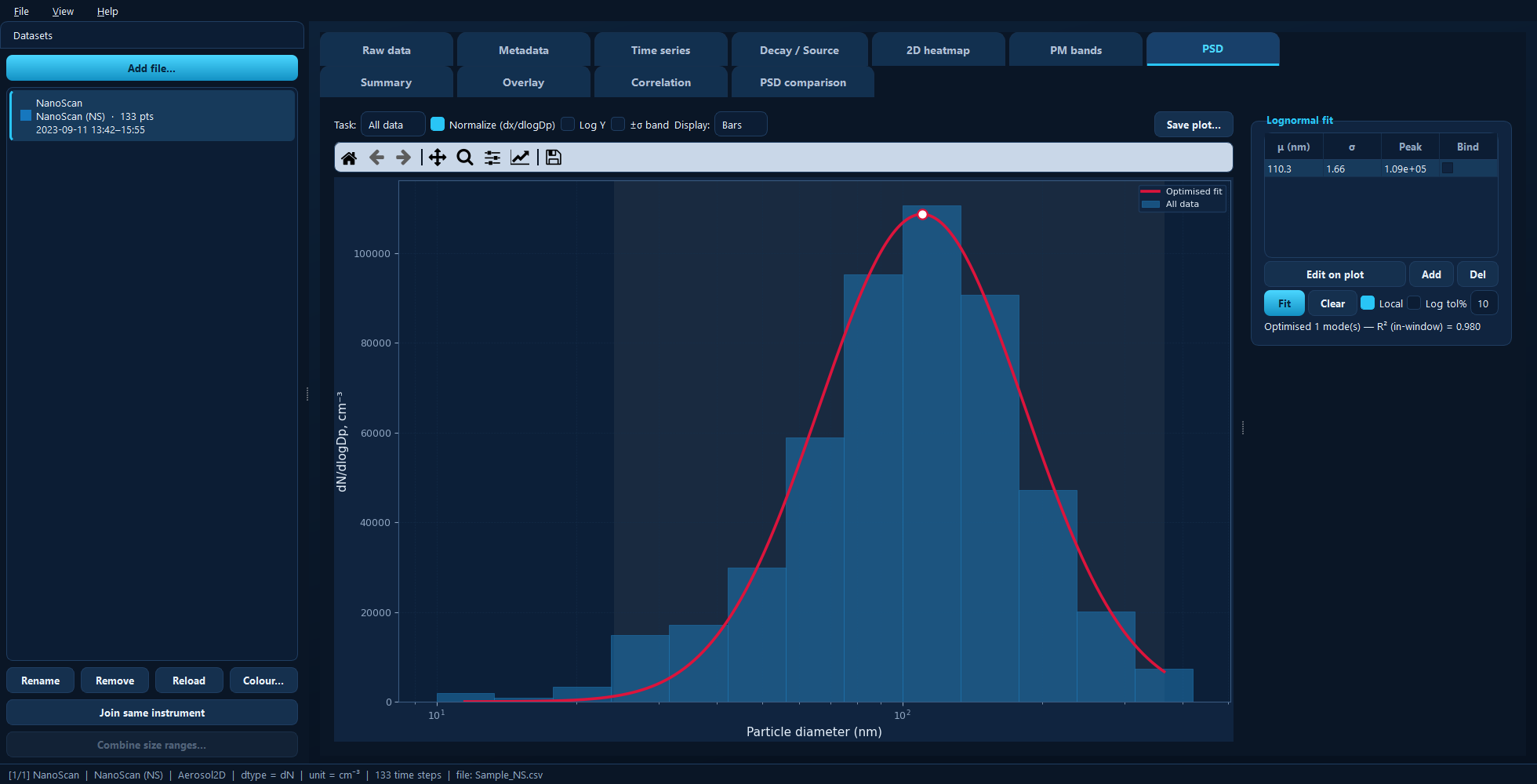
A mean distribution with a single fitted lognormal mode. The fitted µ, σ and peak height appear in the table on the right.
Available for: size-resolved (2D) datasets only.
To compare distributions from several datasets or activities, use PSD comparison instead — this tab deliberately shows one at a time so the fitting stays unambiguous.
Choosing what is shown
Task picks which activity’s mean distribution to show and fit — All data, or any marked activity. Each (dataset × task) keeps its own stored fit, so you can fit one mode set for Sanding and a different one for Background, and both are saved with the project.
Axis appears only for a correlated APS, choosing the aerodynamic or optical distribution.
Display switches between Bars and Lines. Bars show each size bin’s actual width, which is the honest depiction for a single distribution; lines are smoother for reading a fit off.
Normalize (dx/dlogDp) divides each bin by its log-diameter width, so unequal bins are comparable. Lognormal fits are defined in this space, so it is enabled automatically while fitting.
Log Y log-scales the concentration axis; ±σ band shades the spread across the averaged samples, showing how variable the distribution was.
Fitting lognormal modes
A lognormal mode is described by three numbers: the peak diameter µ, the geometric standard deviation σ (its width), and its peak height. The tab lets you place modes by eye and then optimise them.
The typical sequence:
Add puts a mode in the middle of the size range.
Shape it roughly — see below.
Fit optimises it against the shown curve.
To shape a mode by hand, turn on Edit on plot:
With a mode selected, click the plot to set its peak (µ and height), and scroll over the plot to widen or narrow it (σ).
With no mode selected, a click adds a mode there.
You can also type values straight into the table. Del removes the selected mode and Clear removes all modes and the overlay.
Manual and optimised fits are drawn differently, so you can always tell whether what you are looking at has been optimised.
Fitting options
Local (on by default) fits each mode only to the bins near it, in a window scaled by the mode’s width, with the window marked by a shaded band. This keeps each mode on its own peak instead of every mode being pulled towards the largest one.
Log fits against log10(dx/dlogDp) rather than the raw values. It is the right default when a distribution has several modes of very different sizes, because a weak mode would otherwise be swamped by the dominant one.
Tip
With a single dominant mode, try turning Log off. Log weighting spends its effort on the sparse tails and often leaves the curve short of the peak; fitting linearly puts it on the peak instead. On the distribution shown above that is the difference between R² = 0.90 and R² = 0.98.
Bind (a column in the mode table) holds that mode’s µ near its current value during the fit, and tol% sets how far — in percent — a bound µ is allowed to move. Use it when you know a mode’s diameter from elsewhere and want the fit to respect it.
The status line under the buttons reports the result, for example
Optimised 1 mode(s) — R² (in-window) = 0.980.
Tip
If a fit will not settle, check the edge bins first. Instruments are often unreliable in their first or last bin, and one bad edge bin distorts the whole fit. Drop them with Crop size bins on the Metadata tab.
Under the hood
import aerosoltools as at

data = at.load_ns_file("measurement.csv")
result = data.fit_psd(
    period="All data",     # Task
    mu=[113],              # starting peak diameter, nm
    sigma=[1.64],          # starting width
    log_scaling=False,     # the Log checkbox
    tolerance=10.0,        # tol%
)
data.plot_psd()
See 8 — PSD fitting.