Correlation
Compares two datasets measuring the same thing: do they agree, and if not, how do they differ? Two views of that question — a regression and a Bland–Altman agreement plot — plus the option to turn the result into a calibration.
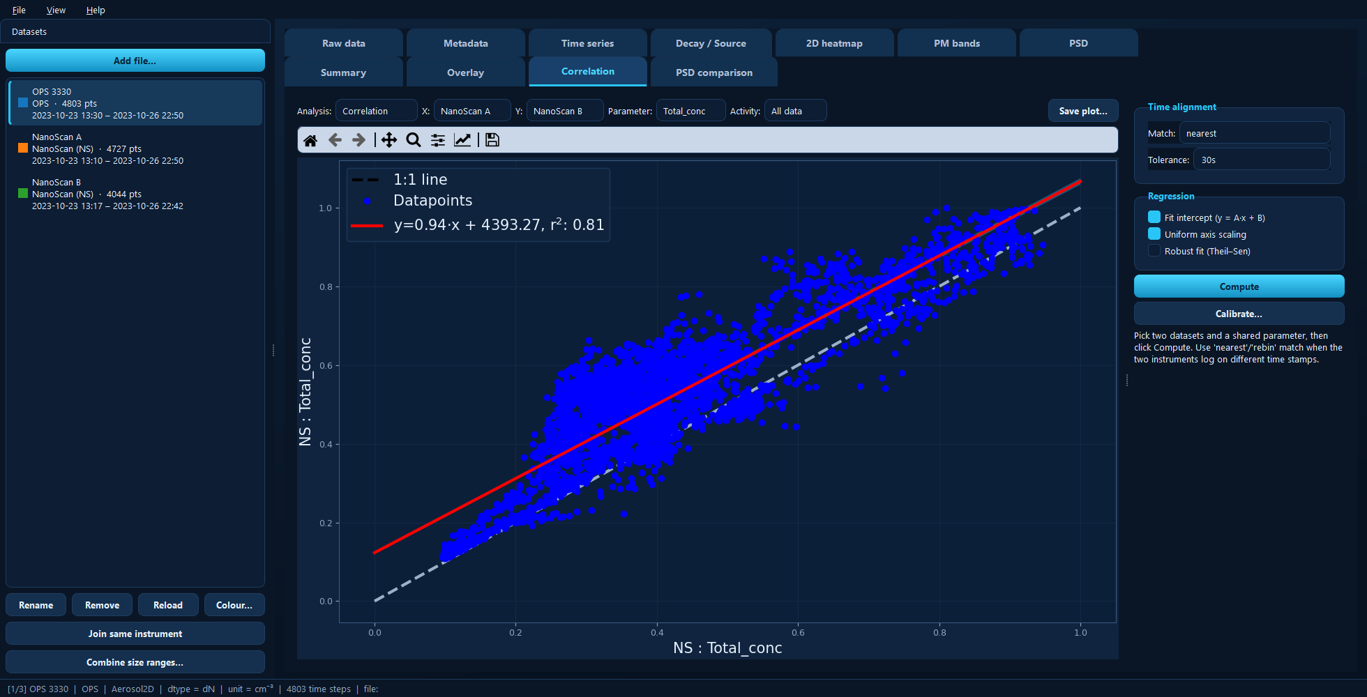
Two NanoScans over the same campaign: y = 0.94·x + 4393, r² = 0.81. The dashed line is 1:1; the red line is the fit.
Available for: projects with at least two datasets that share a parameter.
Choosing the pair
X and Y pick the two datasets, and Parameter picks the quantity they have in common. Which one goes on X matters if you intend to calibrate: the X dataset is treated as the reference.
Activity restricts the comparison to one marked activity. This is more useful than it sounds — instruments often agree well while they are side by side and badly outside that period, and marking the side-by-side window on the Time series tab lets you compare only the part that is a fair test.
Nothing is computed until you press Compute.
Time alignment
Two instruments almost never log on the same timestamps, so the points have to be paired first. Match decides how:
Mode |
Pairing |
Use when |
|---|---|---|
exact |
identical timestamps only |
both instruments log on the same clock |
nearest |
each X point takes the closest Y point within Tolerance |
the usual case — different clocks, similar rates |
rebin |
both are re-binned onto a common time step |
the two log at very different rates |
Tolerance is the largest separation nearest will accept, 30s by default.
For rebin, a common time step (for example 1min; blank = automatic) and
an aggregation method appear.
Tip
An empty or near-empty plot almost always means the alignment, not the data.
With exact and instruments logging a few seconds apart, nothing pairs at all.
Switch to nearest, or raise the tolerance.
Regression options
Fit intercept (y = A·x + B) fits an offset as well as a slope. Untick it to force the line through the origin, which is the right model when you believe the instruments differ only by a scale factor.
Uniform axis scaling gives both axes the same range, so the 1:1 line runs at 45° and deviation from it is visually honest.
Robust fit (Theil–Sen) switches from least squares to the outlier-resistant Theil–Sen estimator. Use it when a handful of spikes are dragging the line around. It drops the confidence band.
Bland–Altman
Setting Analysis to Bland–Altman answers a different question. A regression tells you whether two instruments are related; a Bland–Altman plot tells you whether they can be used interchangeably, by plotting the difference between them against their mean.
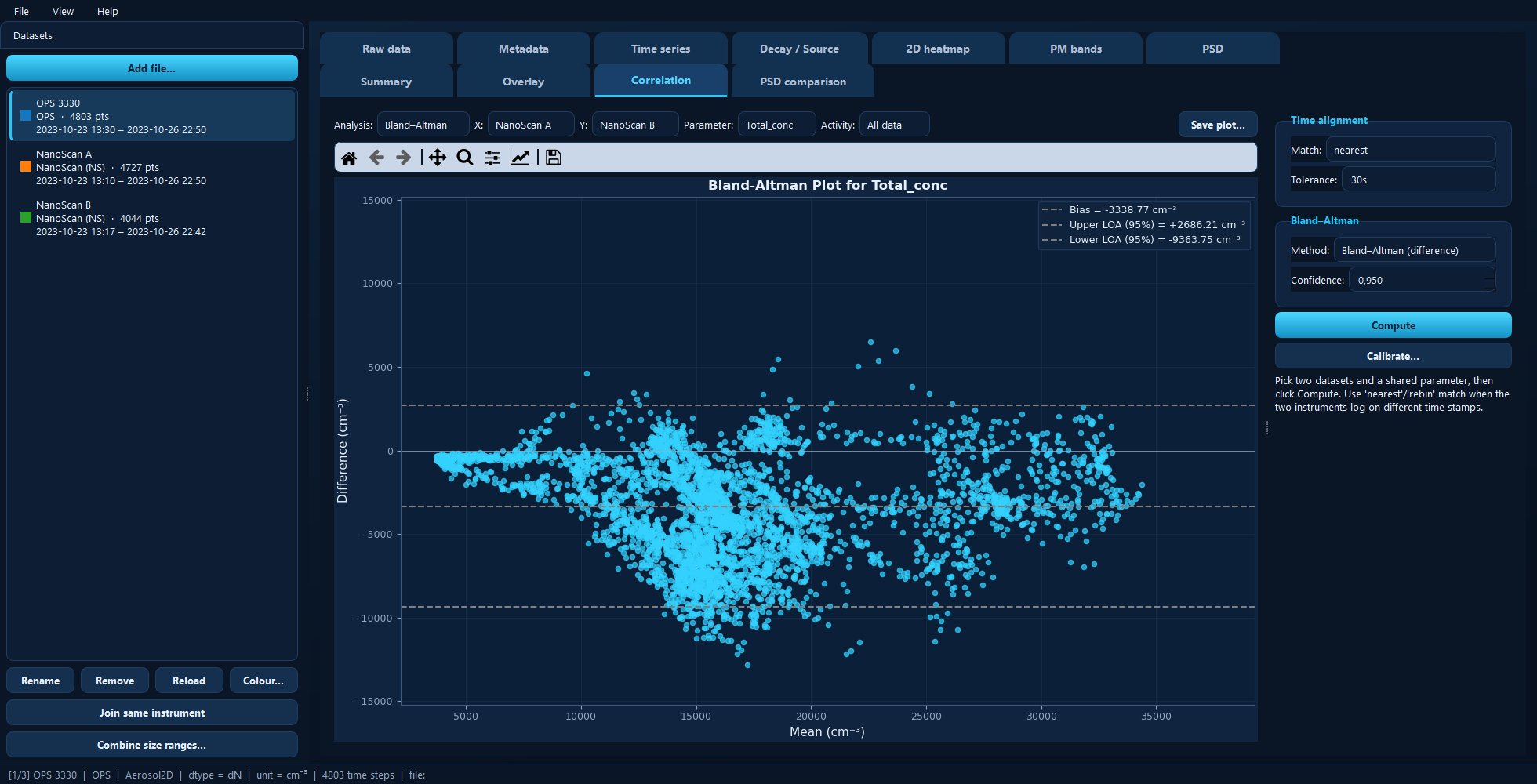
The same pair as a Bland–Altman plot: mean bias and the limits of agreement.
Method chooses the form:
Method |
Plots |
|---|---|
Bland–Altman (difference) |
the raw difference — for a constant offset |
Giavarina (% of mean) |
the difference as a percentage — when the spread grows with concentration |
Euser (log) |
the log-transformed difference — for proportional differences over decades |
Confidence sets the coverage of the limits of agreement, 0.95 by default.
Calibrate…
Turns the comparison into a calibration: it fits a model that makes the Y instrument match the X reference, either on total concentration or bin by bin, and applies it to that one dataset only.
The calibration is fitted on exactly the points the plot shows — same alignment, same activity restriction — so what you see is what you calibrate on. Once applied, it appears in the Calibration group on the Metadata tab, where it can be toggled off or reset.
Under the hood
import aerosoltools as at

a = at.load_ns_file("nanoscan_a.csv")
b = at.load_ns_file("nanoscan_b.csv")

at.plot_correlation(a, b, parameter="Total_conc", match="nearest", tolerance="30s")
at.bland_altman_analysis(a, b, parameter="Total_conc", match="nearest")