7 — Combining datasets
Theme: joining data along time, and joining it across size.
Two different operations are easy to confuse:
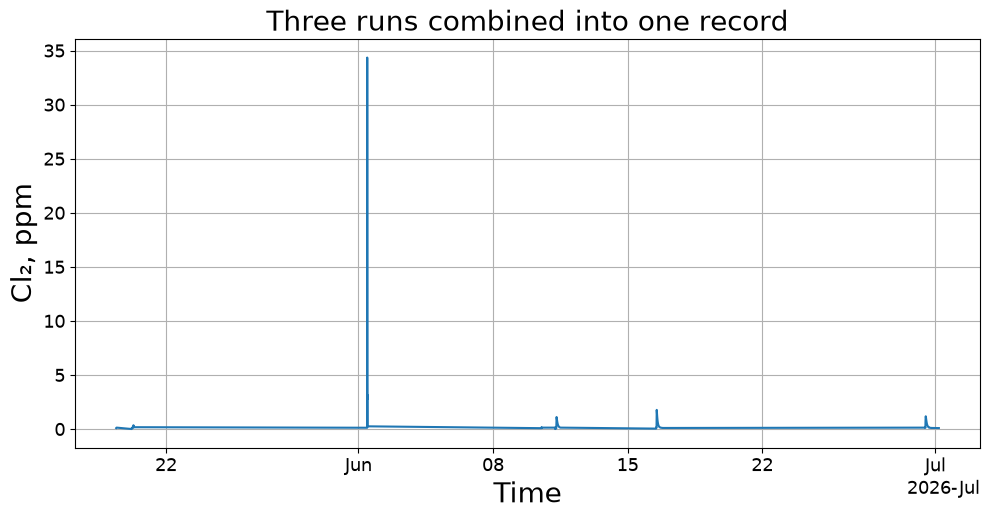
``combine_measurements`` joins runs of the same instrument along the time axis — three days of monitoring into one record.
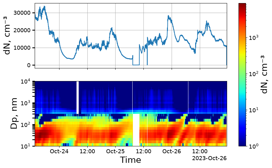
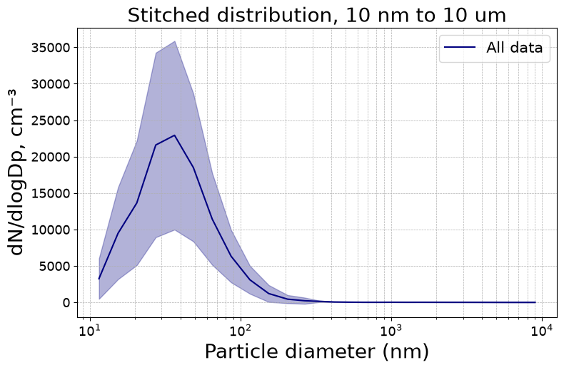
``combine_size_ranges`` joins two different instruments covering neighbouring size ranges into one wider distribution, over the same period.
Both differ from load_data_from_folder, which is about reading many files of one instrument at load time — see 1 — Loading data.
[1]:
import aerosoltools as at
/opt/hostedtoolcache/Python/3.11.15/x64/lib/python3.11/site-packages/tqdm/auto.py:21: TqdmWarning: IProgress not found. Please update jupyter and ipywidgets. See https://ipywidgets.readthedocs.io/en/stable/user_install.html
  from .autonotebook import tqdm as notebook_tqdm
Joining runs along time
A Ranger with interchangeable heads returns one object per measured component, so pick the component you want from each file first.
[2]:
def chlorine(path):
    loaded = at.load_ranger_file(path)
    objects = loaded if isinstance(loaded, list) else [loaded]
    return next(o for o in objects if o.dtype == "Cl₂")


runs = [
    chlorine("../../tests/data/Ranger_2605-1000088-A_20260612-0603.csv"),
    chlorine("../../tests/data/Ranger_2605-1000088-A_20260617-0712.csv"),
    chlorine("../../tests/data/Ranger_2605-1000088-A_20260701-0832.csv"),
]

for run in runs:
    print(f"{len(run.data):5d} samples   {run.time[0]}  ->  {run.time[-1]}")
 1578 samples   2026-05-19 09:44:00  ->  2026-06-11 12:10:00
 1020 samples   2026-06-16 11:24:00  ->  2026-06-17 04:23:00
 2033 samples   2026-06-16 11:24:00  ->  2026-07-01 04:17:00
[3]:
campaign = at.combine_measurements(runs)

print(f"combined: {len(campaign.data)} samples")
print(f"          {campaign.time[0]}  ->  {campaign.time[-1]}")
print(f"          {campaign.dtype} in {campaign.unit}")
combined: 3611 samples
          2026-05-19 09:44:00  ->  2026-07-01 04:17:00
          Cl₂ in ppm
The result is one object of the same class, sorted by time and de-duplicated. Gaps between runs are preserved — nothing is interpolated across them, so a weekend with no measurement stays a hole rather than becoming a straight line.
Note the combined length is smaller than the sum of the inputs: overlapping timestamps are collapsed rather than duplicated.
By default all inputs must share a serial number, which is what stops two different instruments being silently concatenated. Pass require_same_serial=False when the metadata is missing and you know the inputs belong together.
[4]:
fig, ax = campaign.plot_total_conc()
ax.set_title("Three runs combined into one record")
[4]:
Text(0.5, 1.0, 'Three runs combined into one record')
Joining across size
No single instrument covers the whole size range. A NanoScan measures roughly 10–400 nm; an OPS roughly 300 nm–10 µm. combine_size_ranges stitches them into one distribution.
[5]:
ns = at.load_ns_file("../../tests/data/Combine_example_NS.csv")
ops = at.load_data_from_folder(
    "../../tests/data", at.load_ops_file, search_word="Combine_example"
)

print(f"NanoScan: {ns.bin_mids.min():.0f} - {ns.bin_mids.max():.0f} nm")
print(f"OPS     : {ops.bin_mids.min():.0f} - {ops.bin_mids.max():.0f} nm")
Loading files: 100%|██████████| 5/5 [00:00<00:00, 130.91file/s]
File load summary:

+----------------------------------+---------+------------------------------------------------------------------------------------+
|               File               | Status  |                                       Reason                                       |
+----------------------------------+---------+------------------------------------------------------------------------------------+
| Combine_example_OPS - file 1.csv | Loaded  |                                         -                                          |
| Combine_example_OPS - file 2.csv | Loaded  |                                         -                                          |
| Combine_example_OPS - file 3.csv | Loaded  |                                         -                                          |
| Combine_example_OPS - file 4.csv | Loaded  |                                         -                                          |
|      Combine_example_NS.csv      | Skipped | IndexError: too many indices for array: array is 0-dimensional, but 1 were indexed |
+----------------------------------+---------+------------------------------------------------------------------------------------+
NanoScan: 12 - 365 nm
OPS     : 337 - 9016 nm
The two instruments log on different clocks, so they must be aligned in time first. match="nearest" pairs each NanoScan sample with the closest OPS sample within tolerance; match="rebin" puts both onto a common grid instead.
[6]:
combined = at.combine_size_ranges(ns, ops, match="nearest", tolerance="30s")

print(f"combined: {combined.bin_mids.min():.0f} - {combined.bin_mids.max():.0f} nm")
print(f"          {len(combined.bin_mids)} bins, {len(combined.data)} samples")
combined: 12 - 9016 nm
          28 bins, 9582 samples
Where the ranges overlap, one instrument has to win. The crossover diameter decides: bins below it come from the lower instrument, bins above from the upper. Left as None it is chosen automatically; set it explicitly when you have a reason to trust one instrument over the other in the overlap.
The crossover has to lie inside the shared overlap — asking for one outside it raises rather than silently discarding a range.
[7]:
print(f"shared overlap: {ops.bin_mids.min():.0f} - {ns.bin_mids.max():.0f} nm")

low = at.combine_size_ranges(ns, ops, crossover=320, match="nearest", tolerance="30s")
high = at.combine_size_ranges(ns, ops, crossover=400, match="nearest", tolerance="30s")

print(f"crossover 320 nm -> {len(low.bin_mids)} bins")
print(f"crossover 400 nm -> {len(high.bin_mids)} bins")
shared overlap: 337 - 365 nm
crossover 320 nm -> 28 bins
crossover 400 nm -> 27 bins
[8]:
try:
    at.combine_size_ranges(ns, ops, crossover=700, match="nearest", tolerance="30s")
except ValueError as err:
    print("ValueError:", err)
ValueError: crossover 700.0 nm is outside the instruments' shared overlap (300.0-420.0 nm).
The result is an ordinary size-resolved dataset, so everything from the earlier notebooks applies to it.
[9]:
fig, axs = combined.plot_timeseries(y_3d=(1, 0))
[10]:
fig, ax = combined.plot_psd()
ax.set_title("Stitched distribution, 10 nm to 10 um")
[10]:
Text(0.5, 1.0, 'Stitched distribution, 10 nm to 10 um')
Next: 8 — PSD fitting.