Overlay
Several datasets on one time axis — and, if you want, up to three different quantities at once, each on its own y-axis. This is how you check whether two instruments saw the same event, and how you plot quantities whose magnitudes have nothing in common.
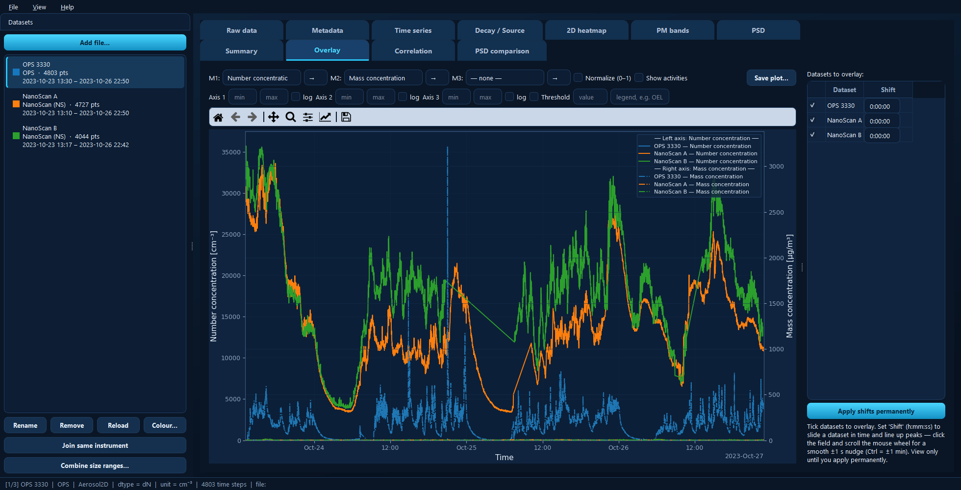
Number concentration (left axis) and mass concentration (right axis) for three datasets. Colour identifies the dataset, line style the metric.
Available for: any project; most useful with two or more datasets.
Reading the plot
Two visual codes, used consistently:
Colour identifies the dataset — the same colour it has in the sidebar and in every other plot. Change it with Colour… in the sidebar.
Line style identifies the metric slot — solid for M1, dash-dot for M2, dotted for M3.
So one dataset shown with two metrics appears twice in its own colour, in two different styles.
Metric slots and axes
M1, M2 and M3 are three independent metric slots. Each can be:
a particle size-distribution total — Number, Mass, Surface area or Volume concentration;
a named measurement, such as a black-carbon or gas channel, listed under its own name;
an instrument-specific extra channel, grouped under its instrument;
or — none — to leave the slot unused.
The → box next to each slot assigns it to a y-axis: 1 = left, 2 = right, 3 = second right. Metrics with different units are never put on the same axis — if you ask for that, the metric is moved to a free or compatible axis automatically.
This is the whole point of the tab. Number concentration in cm⁻³ and mass concentration in µg/m³ differ by orders of magnitude; on one axis the smaller one flattens onto the baseline. On two axes both are readable, as in the screenshot above.
Each axis has its own min, max and log controls.
Normalize (0–1)
Scales every series to the 0–1 range and puts them all on one axis. Magnitudes and units are discarded, leaving only the shape — which is exactly what you want when asking “did these two instruments see the same event?” rather than “did they agree on the value?”
Lining datasets up in time
Instrument clocks drift. The Shift column beside each dataset applies a
view-only time shift as h:mm:ss — for example -0:00:30 moves it 30 seconds
earlier. A bare number is read as seconds.
Click into the field and scroll the mouse wheel to nudge by ±1 s, or Ctrl + scroll for ±1 min, watching the peaks line up as you go.
Nothing is modified while you do this. When the alignment is right, Apply shifts permanently bakes the current shifts into the datasets’ time axes. Shared activities keep their absolute times, so your task marks stay where they were.
Tip
To correct a clock properly — permanently, and before any analysis — use the Time shift control on the Time series tab. The Overlay shift is for finding the offset; the Time series one is for fixing it.
Other controls
Show activities shades the project’s activities across every dataset, so you can see how different instruments behaved within the same task window.
Threshold draws a reference line with an optional legend label.
Under the hood
import aerosoltools as at

a = at.load_ops_file("ops.csv")
b = at.load_ns_file("nanoscan.csv")

b.timeshift(seconds=-30)     # Apply shifts permanently

fig, ax = a.plot_total_conc()
b.plot_total_conc(ax=ax)
See 5 — Plotting and 7 — Combining datasets.