9 — Decay and source fitting
Theme: extracting physical rates from a concentration peak.
When a source runs in a room and then stops, the concentration rises and then decays away. Fitting that shape recovers quantities you cannot read off the plot: how strong the source was, and how fast the room cleared it.
The decay combines ventilation and deposition to surfaces, so the fitted loss rate is the total removal rate.
[1]:
import matplotlib.pyplot as plt
import numpy as np

import aerosoltools as at

ns = at.load_ns_file("../../tests/data/Sample_NS.csv")

fig, ax = ns.plot_total_conc()
ax.set_title("A single release with a clean decay")
/opt/hostedtoolcache/Python/3.11.15/x64/lib/python3.11/site-packages/tqdm/auto.py:21: TqdmWarning: IProgress not found. Please update jupyter and ipywidgets. See https://ipywidgets.readthedocs.io/en/stable/user_install.html
  from .autonotebook import tqdm as notebook_tqdm
[1]:
Text(0.5, 1.0, 'A single release with a clean decay')
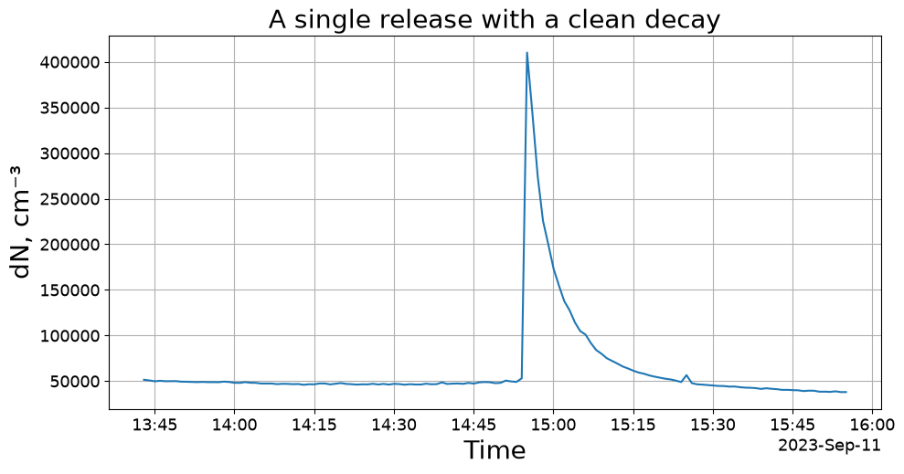
This is the shape the fit expects: a flat background, a sharp rise while the source runs, and a smooth decay once it stops.
[2]:
tc = ns.total_concentration
print(f"background : ~{tc.iloc[:20].mean():,.0f} {ns.unit}")
print(f"peak       : {tc.max():,.0f} {ns.unit} at {tc.idxmax()}")
print(f"enhancement: {tc.max() / tc.iloc[:20].mean():.1f}x above background")
background : ~49,425 cm⁻³
peak       : 410,173 cm⁻³ at 2023-09-11 14:55:04
enhancement: 8.3x above background
Fitting the peak
fit_decay takes the window containing the event — as a (start, end) pair or the name of a marked activity. The window should start before the rise and end while the decay is still visible above the noise.
[3]:
window = ("2023-09-11 14:45:00", "2023-09-11 15:35:00")

fit = ns.fit_decay(period=window, metric="PNC")

print("model          :", fit.model)
print("points fitted  :", fit.n_points)
print(f"R^2 (whole)    : {fit.r_squared:.4f}")
print(f"R^2 (decay)    : {fit.decay_r_squared:.4f}")
model          : combined
points fitted  : 50
R^2 (whole)    : 0.8861
R^2 (decay)    : 0.9973
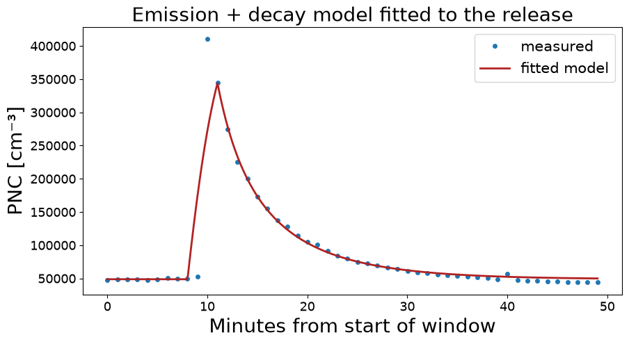
Two R² values are reported because the curve has two stages. The decay stage is usually the better-determined one — the rise depends on exactly when the source started and stopped, which is often uncertain.
Seeing the fit
decay_curve rebuilds the modelled curve from model and model_popt, so the fit can be drawn over the data it came from.
[4]:
measured = ns.total_concentration.loc[window[0]:window[1]]
seconds = (measured.index - fit.window_start).total_seconds()

t = np.linspace(0, seconds.max(), 500)
modelled = at.decay_curve(fit.model, t, fit.model_popt)

fig, ax = plt.subplots(figsize=(10, 5))
ax.plot(seconds / 60, measured.values, "o", ms=4, color="tab:blue",
        label="measured")
ax.plot(t / 60, modelled, "-", lw=2, color="firebrick", label="fitted model")
ax.set_xlabel("Minutes from start of window")
ax.set_ylabel(f"PNC [{fit.unit}]")
ax.legend()
ax.set_title("Emission + decay model fitted to the release")
[4]:
Text(0.5, 1.0, 'Emission + decay model fitted to the release')
What the fit found
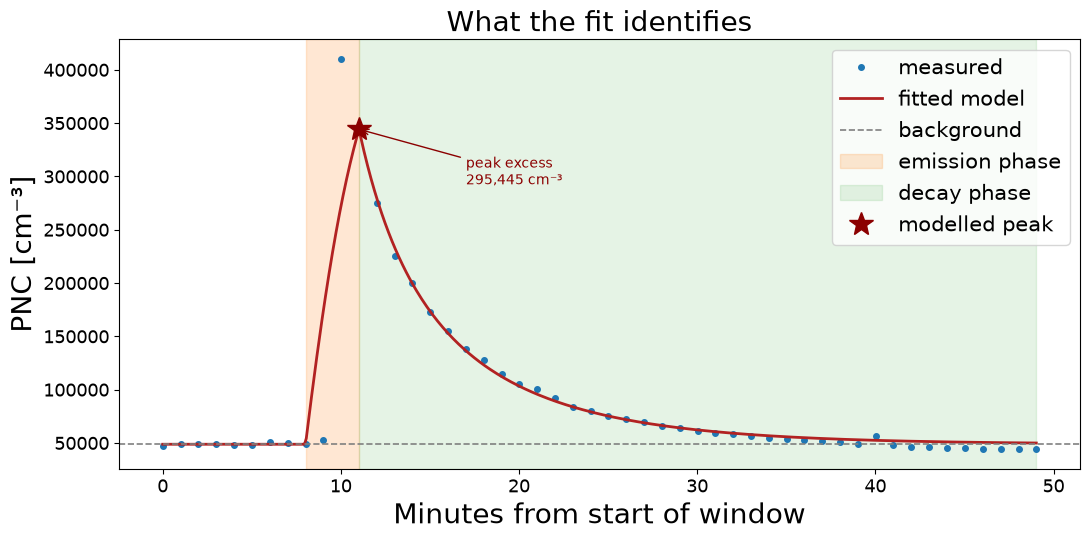
The fit splits the curve into a background, an emission phase and a decay, and reports where each begins.
[5]:
print(f"background         : {fit.background:>12,.0f} {fit.unit}")
print(f"modelled peak      : {fit.peak_concentration:>12,.0f} {fit.unit}")
print(f"peak excess        : {fit.peak_excess:>12,.0f} {fit.unit}")
print()
print(f"emission starts at : {fit.emission_start_s / 60:>6.1f} min into the window")
print(f"emission lasts     : {fit.emission_duration_s / 60:>6.1f} min")
print(f"peak reached at    : {fit.peak_time_s / 60:>6.1f} min  ({fit.peak_time})")
background         :       48,782 cm⁻³
modelled peak      :      344,227 cm⁻³
peak excess        :      295,445 cm⁻³

emission starts at :    8.0 min into the window
emission lasts     :    3.0 min
peak reached at    :   11.0 min  (2023-09-11 14:56:04)
Marking those on the plot shows what each number refers to.
[6]:
fig, ax = plt.subplots(figsize=(11, 5.5))

ax.plot(seconds / 60, measured.values, "o", ms=4, color="tab:blue", label="measured")
ax.plot(t / 60, modelled, "-", lw=2, color="firebrick", label="fitted model")

# background level
ax.axhline(fit.background, ls="--", color="gray", lw=1.2, label="background")

# the emission phase
ax.axvspan(fit.emission_start_s / 60,
           (fit.emission_start_s + fit.emission_duration_s) / 60,
           color="tab:orange", alpha=0.18, label="emission phase")

# the decay phase
ax.axvspan(fit.peak_time_s / 60, seconds.max() / 60,
           color="tab:green", alpha=0.12, label="decay phase")

# the peak
ax.plot(fit.peak_time_s / 60, fit.peak_concentration, "*", ms=18,
        color="darkred", label="modelled peak", zorder=5)

ax.annotate(
    f"peak excess\n{fit.peak_excess:,.0f} {fit.unit}",
    xy=(fit.peak_time_s / 60, fit.peak_concentration),
    xytext=(fit.peak_time_s / 60 + 6, fit.peak_concentration * 0.85),
    arrowprops=dict(arrowstyle="->", color="darkred"),
    color="darkred",
)

ax.set_xlabel("Minutes from start of window")
ax.set_ylabel(f"PNC [{fit.unit}]")
ax.legend(loc="upper right")
ax.set_title("What the fit identifies")
plt.tight_layout()
The decay rate
The decay rate is the physically interesting output: how quickly the room removes particles, by ventilation and deposition together.
[7]:
print(f"decay rate : {fit.decay_rate:.6f} per second")
print(f"           : {fit.decay_rate_per_hour:.3f} per hour")
print(f"half-life  : {fit.half_life_hours * 60:.1f} minutes")
decay rate : 0.002108 per second
           : 7.589 per hour
half-life  : 5.5 minutes
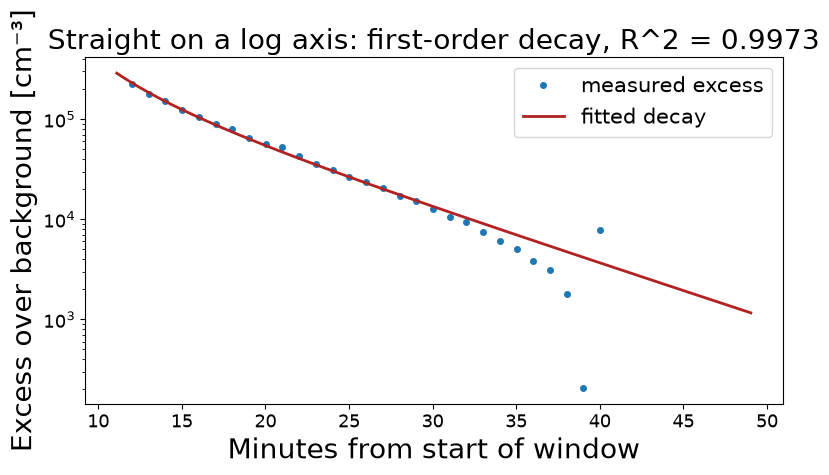
On a log scale a first-order decay is a straight line, which is the quickest visual check that the model is appropriate.
[8]:
after_peak = seconds > fit.peak_time_s

fig, ax = plt.subplots(figsize=(9, 4.5))
ax.semilogy(seconds[after_peak] / 60,
            measured.values[after_peak] - fit.background,
            "o", ms=4, color="tab:blue", label="measured excess")

t_decay = t[t > fit.peak_time_s]
ax.semilogy(t_decay / 60,
            at.decay_curve(fit.model, t_decay, fit.model_popt) - fit.background,
            "-", lw=2, color="firebrick", label="fitted decay")

ax.set_xlabel("Minutes from start of window")
ax.set_ylabel(f"Excess over background [{fit.unit}]")
ax.legend()
ax.set_title(f"Straight on a log axis: first-order decay, R^2 = {fit.decay_r_squared:.4f}")
[8]:
Text(0.5, 1.0, 'Straight on a log axis: first-order decay, R^2 = 0.9973')
Source strength
An emission rate in concentration per second only becomes a source strength once you know the volume it filled — the same source in a smaller room drives a larger concentration. Supply volume in cubic metres.
[9]:
fit_v = ns.fit_decay(period=window, metric="PNC", volume=30.0)

print(f"emission rate  : {fit_v.emission_rate:,.1f} {fit_v.emission_rate_unit}")
print(f"source strength: {fit_v.source_strength:.3e} particles/s")
print(f"total emitted  : {fit_v.total_emitted:.3e} particles")
emission rate  : 2,271.6 cm⁻³/s
source strength: 6.815e+10 particles/s
total emitted  : 1.227e+13 particles
Separating ventilation from deposition
The fitted decay lumps together air exchange and losses to surfaces. Given the air exchange rate independently — from a tracer-gas measurement, or the ventilation setpoint — the wall-loss term is reported separately.
[10]:
split = ns.fit_decay(period=window, metric="PNC", volume=30.0,
                     air_exchange_rate=2.0)

print(f"total decay  : {split.decay_rate_per_hour:.3f} per hour")
print(f"air exchange : 2.000 per hour (given)")
print(f"wall loss    : {split.wall_loss_rate_per_hour:.3f} per hour")
total decay  : 7.589 per hour
air exchange : 2.000 per hour (given)
wall loss    : 5.589 per hour
The split is arithmetic, not fitted — the model cannot tell the two apart from the decay alone, so the air exchange rate you supply is taken at face value.
The window matters
Extending the window into the noise, or cutting it short, changes the answer. Compare three choices:
[11]:
for start, end in [("2023-09-11 14:45:00", "2023-09-11 15:35:00"),
                   ("2023-09-11 14:45:00", "2023-09-11 15:15:00"),
                   ("2023-09-11 14:45:00", "2023-09-11 15:55:00")]:
    f = ns.fit_decay(period=(start, end), metric="PNC")
    print(f"{start[-8:]} - {end[-8:]}   "
          f"decay {f.decay_rate_per_hour:6.3f} /h   "
          f"decay R^2 {f.decay_r_squared:.4f}   n={f.n_points}")
14:45:00 - 15:35:00   decay  7.589 /h   decay R^2 0.9973   n=50
14:45:00 - 15:15:00   decay  7.511 /h   decay R^2 0.9987   n=30
14:45:00 - 15:55:00   decay  7.721 /h   decay R^2 0.9904   n=70
Fitting a marked activity
If the event is already marked, pass the activity name instead of a time pair.
[12]:
ns.mark_activities({"Release": [window]})

by_name = ns.fit_decay(period="Release", metric="PNC")
print(f"decay {by_name.decay_rate_per_hour:.3f} per hour, "
      f"R^2 {by_name.decay_r_squared:.4f}")
decay 7.574 per hour, R^2 0.9974
Fitting a different metric
metric accepts anything summarize_exposure accepts. Mass-based metrics decay faster than number, because they are dominated by larger particles that settle out.
[13]:
for metric in ["PNC", "PM1", "PM10"]:
    f = ns.fit_decay(period=window, metric=metric)
    print(f"{metric:5s} decay {f.decay_rate_per_hour:6.3f} /h   "
          f"half-life {f.half_life_hours * 60:5.1f} min")
PNC   decay  7.589 /h   half-life   5.5 min
PM1   decay  7.961 /h   half-life   5.2 min
PM10  decay  7.972 /h   half-life   5.2 min