PSD comparison
Mean size distributions from several datasets and activities, overlaid on one axis. Use it to answer questions like did sanding produce finer particles than cleaning? or do these two instruments see the same distribution?
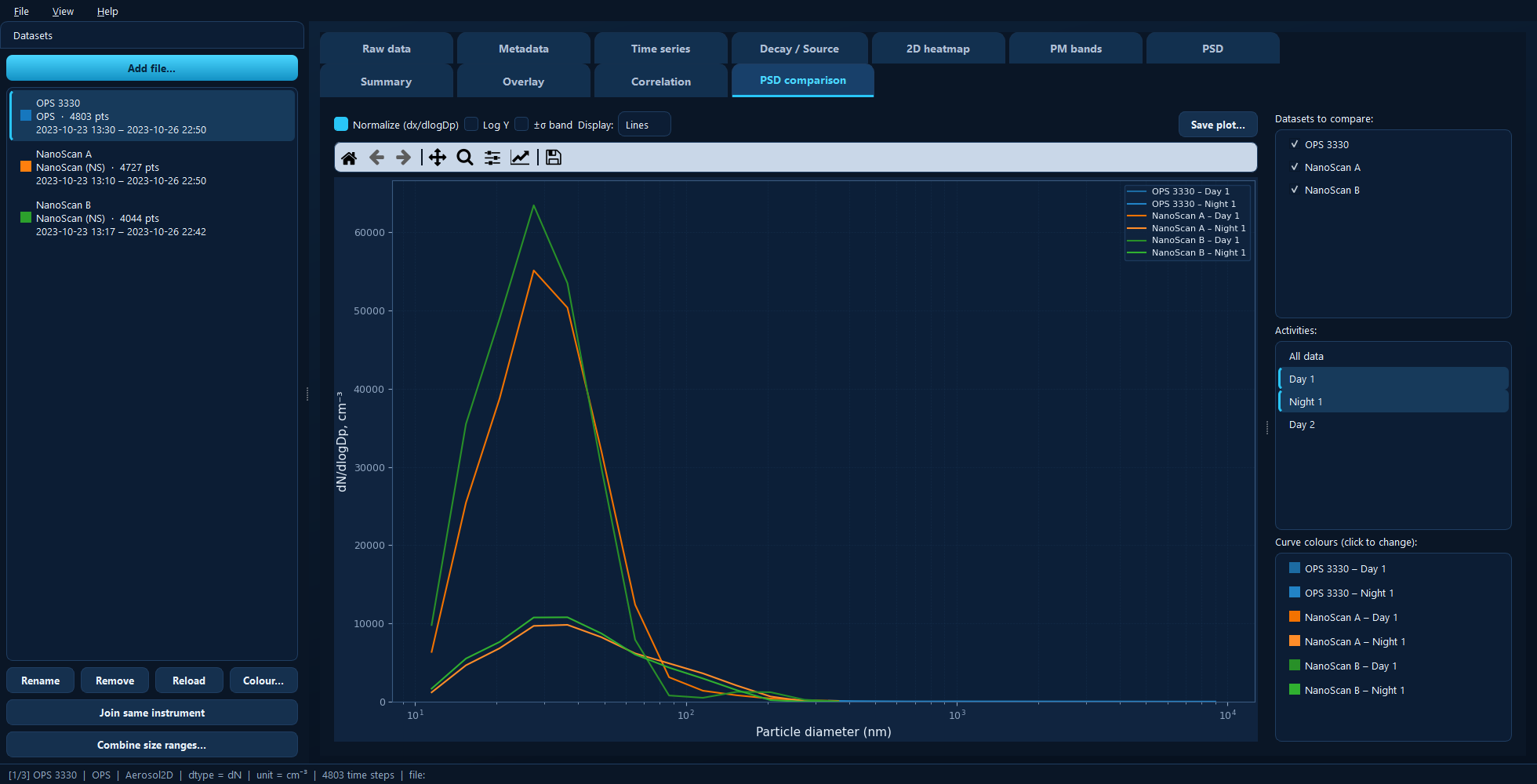
One curve per ticked dataset × selected activity, each in its own shade, with the colour list on the right.
Available for: projects containing size-resolved (2D) datasets. Only those appear in the list.
This pane is display only — there is no fitting here. Lognormal fitting lives on the PSD tab, which shows one distribution at a time so the fitting rules stay simple.
Choosing the curves
Datasets to compare ticks which datasets take part; Activities is a multi-select list of periods, defaulting to All data.
One curve is drawn per dataset × activity combination, so two datasets and two activities give four curves. That grid is the point of the tab: it lets you separate an instrument effect from a task effect in one picture.
Combinations that do not exist — an activity that does not apply to a given dataset — are simply skipped.
Curve colours
The list on the right has one row per drawn curve. Each activity defaults to a shade of its dataset’s colour, so curves from the same instrument stay visually grouped while remaining distinguishable. Click any row to pick a custom colour; the choice is saved with the project.
Display options
Display switches between Lines and Bars. Lines are clearer when several curves share the axes — which is the normal case here. Bars show each bin’s true width, and are better for a single distribution (see the PSD tab).
Normalize (dx/dlogDp) divides each bin by its log-diameter width. Keep it on when comparing different instruments: their size bins are not the same width, and without normalisation you are comparing binning choices as much as aerosol.
Log Y log-scales the concentration axis, useful when the distributions differ by orders of magnitude.
±σ band shades each curve’s ±1σ spread. It is off by default for a good reason — with several curves the bands overlap heavily and obscure everything. Turn it on when comparing two curves and you need to know whether a difference is larger than the variability.
Under the hood
import matplotlib.pyplot as plt
import aerosoltools as at

a = at.load_ops_file("ops.csv")
b = at.load_ns_file("nanoscan.csv")

fig, ax = plt.subplots()
a.plot_psd(activities=["Sanding"], normalize=True, ax=ax)
b.plot_psd(activities=["Sanding"], normalize=True, ax=ax)
See 8 — PSD fitting and 7 — Combining datasets.