Summary
Turns marked activities into numbers: mean concentration per task, and exposure metrics against occupational limits. This is usually the tab you came for — the one whose table ends up in the report.
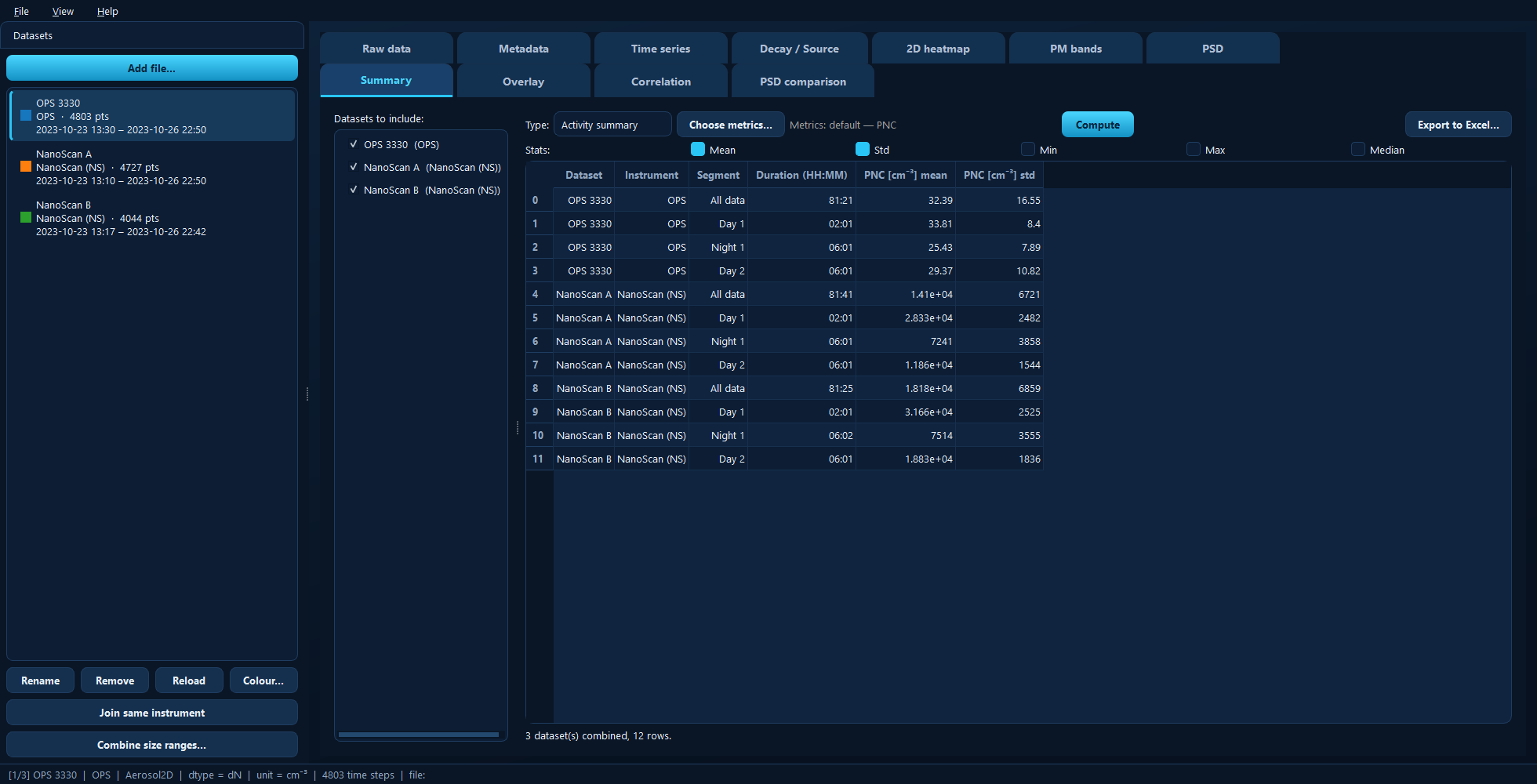
One row per dataset × activity, with the statistics you asked for. Several instruments are combined into a single table.
Available for: any project. It works with one dataset or many — tick several
and they are combined into one table with Dataset and Instrument columns, so
you can compare instruments task by task.
Mark your activities on the Time series tab first; with none marked you only get an All data row.
Datasets to include
Tick the datasets to summarise. Nothing is computed until you press Compute, because exposure statistics over several long datasets can take a moment.
Type
Activity summary — descriptive statistics per activity: duration plus whichever of Mean, Std, Min, Max and Median you tick.
Exposure summary — the occupational-hygiene view: the time-weighted average over the TWA window, the highest short-term average, peaks, and how each compares against the limits you set. It reveals the extra fields:
Field |
Meaning |
|---|---|
STEL (short-term limit) |
Short-term exposure limit. The highest short-window average is compared against it. |
over |
Averaging window for the STEL check, as a pandas offset — |
OEL (8h limit) |
Occupational exposure limit. The time-weighted average is compared against it. |
TWA window |
Averaging window for the time-weighted average — |
Both limits are in the same unit as the metric you chose, so if you are summarising a mass concentration in µg/m³, enter the limit in µg/m³.
Choose metrics…
Picks which quantities to summarise, grouped by instrument. Two things make this work across a mixed project:
Each metric is computed only for the datasets that provide it, so adding a gas monitor to a project full of particle counters does not fill the table with blanks.
Comparable quantities recorded at different unit scales — ng/m³ and µg/m³, say — are merged into one column.
Compute, and the staleness warning
Compute builds the table. The result is cached and saved with the project, so reopening it later shows what you computed without recalculating.
Because it is cached, it can go out of date. If you edit activities, change the data, or alter any of the limits, an amber banner appears:
⚠ These values may be out of date — tasks, data, or settings changed since they were computed. Click Compute to refresh.
Take it seriously — the numbers shown were computed from the previous inputs.
Export to Excel…
Writes the combined table to .xlsx or .csv, exactly as displayed.
Under the hood
import aerosoltools as at

data = at.load_ops_file("measurement.csv")

# Activity summary
data.summarize_activities(stats=["mean", "std"])

# Exposure summary
data.summarize_exposure(
    metric="PM4.2",
    long_limit=1.0,       # OEL (8h limit)
    twa_window="8h",      # TWA window
    short_limit=1.0,      # STEL
    short_window="15min", # over
)