Time series
Concentration over time for the active dataset, and the place where you do three things: mark what happened when, clean the data up, and cut it into pieces. Most sessions start here.
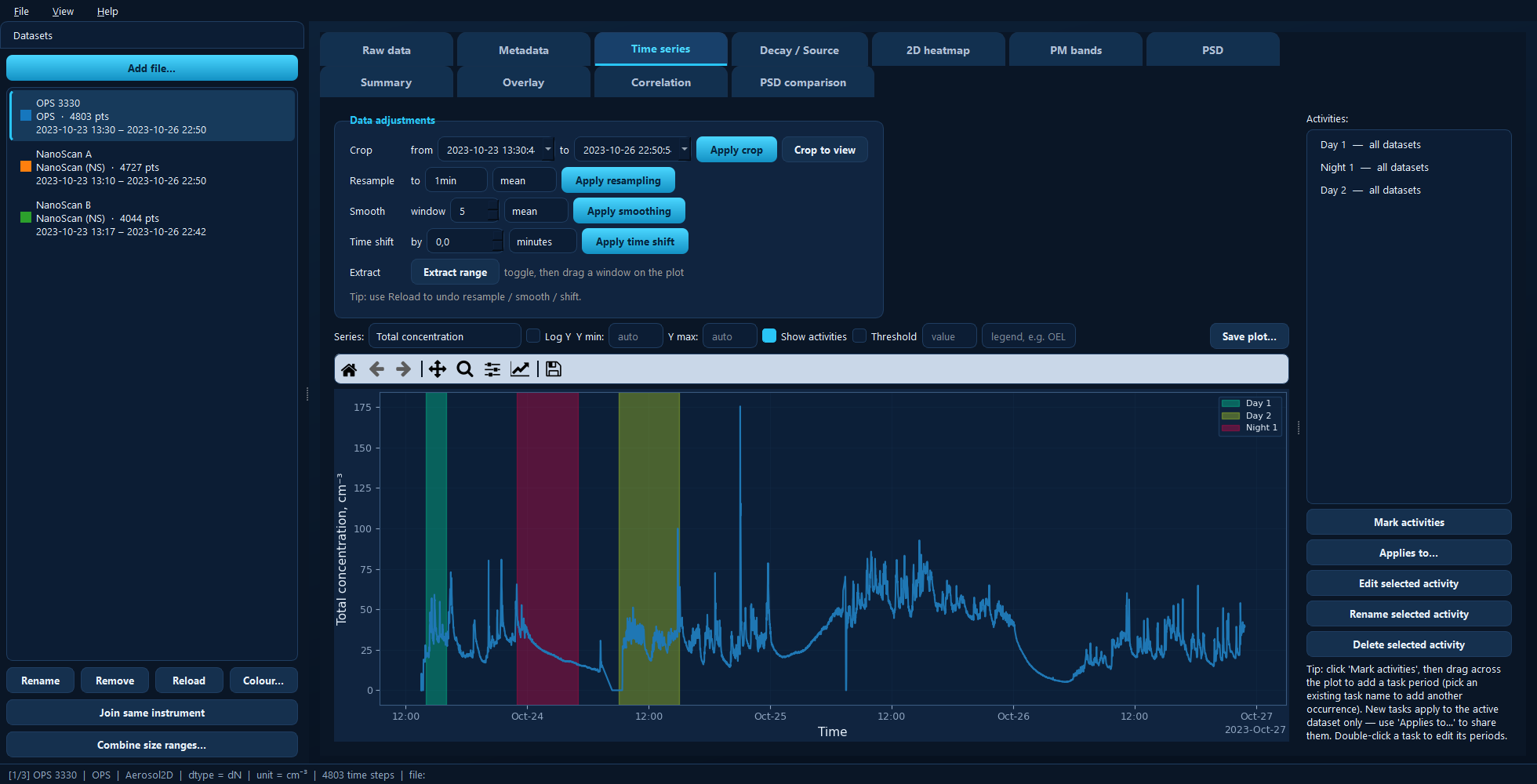
Three marked activities shaded on the trace, the data-adjustment controls above, and the activities list on the right.
Available for: every dataset.
Choosing what to plot
Series picks the line. You always get Total concentration; size-resolved instruments additionally offer mass, surface-area and volume concentration, and any auxiliary channels the instrument logged appear below an Extra heading.
Log Y switches the y-axis to logarithmic — usually the right choice when a peak is orders of magnitude above the background. Y min / Y max override the automatic limits; leave them blank for auto.
Show activities shades the marked periods, each in its own colour with a legend.
Threshold draws a horizontal reference line — an occupational exposure limit,
say. Enter the value and, optionally, a label for the legend such as OEL.
Scroll to zoom, right-drag to pan, and use the toolbar’s home button to get back.
Marking activities
This is the core workflow of the whole application.
Click Mark activities to arm it.
Drag across the plot over the period you want.
Name it — or pick an existing name from the list to add another occurrence of the same task.
The marked period appears shaded, and the task joins the Activities list on the right. One task can have as many separate occurrences as you like; they are all reported together.
A new task applies to the active dataset only. That is deliberate — you often mark on the instrument where the event is clearest. To share it:
Applies to… — choose whether the selected task covers all datasets or a chosen subset. Because activities are stored in absolute time, every instrument that was running then picks up the same window.
The remaining buttons act on the task selected in the list:
Edit selected activity — open its periods for editing. You can Add period, Remove selected, and adjust the start and end times by hand. Double-clicking a task in the list does the same thing.
Rename selected activity — rename it everywhere it applies.
Delete selected activity — remove it from the project.
Each entry in the list is annotated with the datasets it applies to, so you can see and manage scoped tasks from any dataset.
Adjusting the data
The Data adjustments panel sits above the plot so that processing happens where you can see its effect.
Crop — keep only the data between two timestamps. Type them, or click Crop to view to crop to whatever you have currently zoomed to, which is usually faster.
Resample — change the time step (1min, 30s, …) with an aggregation of
mean, median, min, max or sum. Use it to bring instruments logging at
different rates onto a comparable footing, or to thin out a very long record.
Smooth — a rolling window over a number of samples, again with a choice of aggregation. Useful for a noisy trace, but remember it flattens short peaks.
Time shift — move the whole record forwards or backwards. This is how you fix an instrument whose clock was wrong. (To line datasets up visually without changing them, use the shift column on the Overlay tab instead.)
Tip
Reload in the sidebar re-reads the source file, undoing resampling, smoothing and time shifts. There is no undo stack, so Reload is your safety net.
Cutting a dataset up
Extract range toggles extraction on; then drag a window on the plot. What happens next depends on one checkbox:
Copy the window to a new dataset (keep the original) ticked — the window is copied into a new dataset under the name you give, and the original is left alone. Good for pulling one interesting event out for closer study.
Unticked — the dataset is split at the window edges: the data before the window, the window itself, and the data after it each become a separate dataset, and the original is removed. A window in the middle gives three datasets; one touching an end gives two.
Either way the new datasets inherit the activities that apply to them.
Under the hood
import aerosoltools as at

data = at.load_ops_file("measurement.csv")
data.mark_activities({"Sanding": [("2023-10-23 14:00", "2023-10-23 16:00")]})
data.timecrop("2023-10-23 13:30", "2023-10-26 22:50")
data.timerebin("1min")        # Resample
data.timesmooth(5)            # Smooth
data.timeshift(-30)           # Time shift
data.plot_timeseries()
See 2 — Time adjustments, 3 — Activities and 5 — Plotting.