6 — Dtypes, density and corrections
Theme: changing what the numbers mean before analysing them.
A size distribution can be expressed as number, surface, volume or mass; mass depends on an assumed particle density; and a sampling line removes some of the smallest particles before they are ever counted. This notebook covers those conversions and corrections, plus the derived PM fractions built on top of them.
[1]:
import aerosoltools as at

elpi = at.load_elpi_file("../../tests/data/Sample_ELPI.txt")
print("dtype  :", elpi.dtype)
print("unit   :", elpi.unit)
print("density:", elpi.density, "g/cm3")
dtype  : dN
unit   : cm⁻³
density: 0.14 g/cm3
/opt/hostedtoolcache/Python/3.11.15/x64/lib/python3.11/site-packages/tqdm/auto.py:21: TqdmWarning: IProgress not found. Please update jupyter and ipywidgets. See https://ipywidgets.readthedocs.io/en/stable/user_install.html
  from .autonotebook import tqdm as notebook_tqdm
/home/runner/work/aerosoltools/aerosoltools/src/aerosoltools/loaders/elpi.py:525: RuntimeWarning: ELPI density is not 1.0 g/cm3; bin edges were estimated from geometric means of CalculatedDi values.
  return load_elpi_file_txt(
The warning on load is the point of this notebook: the file records a particle density other than 1.0 g/cm³, and every mass-based quantity depends on it.
Distribution types
dtype records what the numbers are. dtype_converter converts between them:
dtype |
quantity |
|---|---|
|
number |
|
surface area |
|
volume |
|
mass |
The conversion is geometric — number to volume uses the bin diameters, volume to mass multiplies by density — so it only makes sense on size-resolved data.
[2]:
mass = elpi.copy_self()
mass.dtype_converter("dM")
print("dtype:", mass.dtype)
print("unit :", mass.unit)
dtype: dM
unit : µg/m³
[3]:
surface = elpi.copy_self()
surface.dtype_converter("dS")
print("dtype:", surface.dtype, "| unit:", surface.unit)
dtype: dS | unit: nm²/cm³
Density
Mass is number × volume × density, so an assumed density propagates into every mass result. set_density changes it.
[4]:
denser = elpi.copy_self()
denser.set_density(2.0)
denser.dtype_converter("dM")

print(f"density 1.5 -> mean mass {mass.total_concentration.mean():.1f} {mass.unit}")
print(f"density 2.0 -> mean mass {denser.total_concentration.mean():.1f} {denser.unit}")
density 1.5 -> mean mass 124.6 µg/m³
density 2.0 -> mean mass 148.2 µg/m³
Density is an assumption unless you have measured it. Reporting the value you used matters as much as the result.
For the ELPI specifically, density also affects the size axis itself: the aerodynamic diameters the instrument reports are recomputed when you call set_density, because a denser particle of the same aerodynamic size is physically smaller.
Per-column dtypes and units
Multi-channel instruments carry a dtype and unit per column. dtype_of and unit_of answer for one column.
[5]:
dust = at.load_dusttrak_file("../../tests/data/Sample_DustTrak.csv")

print("PM1  ->", dust.dtype_of("PM1"), dust.unit_of("PM1"))
print("PM10 ->", dust.dtype_of("PM10"), dust.unit_of("PM10"))
print()
print("all columns:", dust.column_units)
PM1  -> dM µg/m³
PM10 -> dM µg/m³

all columns: {}
dlogDp normalisation
Instruments use different bin widths, so raw per-bin concentrations are not comparable between them. Dividing by the width of each bin in log space gives dN/dlogDp, which is.
[6]:
norm = elpi.copy_self()
norm.normalize_logdp()
print("normalised   :", norm.dtype)

norm.unnormalize_logdp()
print("back to base :", norm.dtype)
normalised   : dN/dlogDp
back to base : dN
Most plotting and fitting works on the normalised form — plot_psd normalises by default — so you rarely call these directly. They matter when you are exporting numbers for something else, or comparing against data that has already been normalised.
Size bins
The bin structure is available directly.
[7]:
print("number of bins:", len(elpi.bin_mids))
print("first mids  [nm]:", elpi.bin_mids[:5].round(1))
print("first edges [nm]:", elpi.bin_edges[:6].round(1))
number of bins: 14
first mids  [nm]: [ 22.6  88.8 128.7 190.4 287. ]
first edges [nm]: [ 18.8  44.8 106.9 156.5 233.8 362.7]
rebin_bin_edges maps the distribution onto a different set of edges — needed when two instruments must share a size axis before they can be combined or compared.
[8]:
elpi.size_data.iloc[:3, :5]
[8]:
| 22.6 | 88.8 | 128.7 | 190.4 | 287.0 | |
|---|---|---|---|---|---|
| Datetime | |||||
| 2023-09-07 09:06:38 | 0.000 | 26.76 | 21.14 | 31.25 | 36.22 |
| 2023-09-07 09:06:39 | 10.790 | 23.07 | 21.32 | 30.06 | 35.63 |
| 2023-09-07 09:06:40 | 5.988 | 23.08 | 19.76 | 30.23 | 35.89 |
Diffusion losses
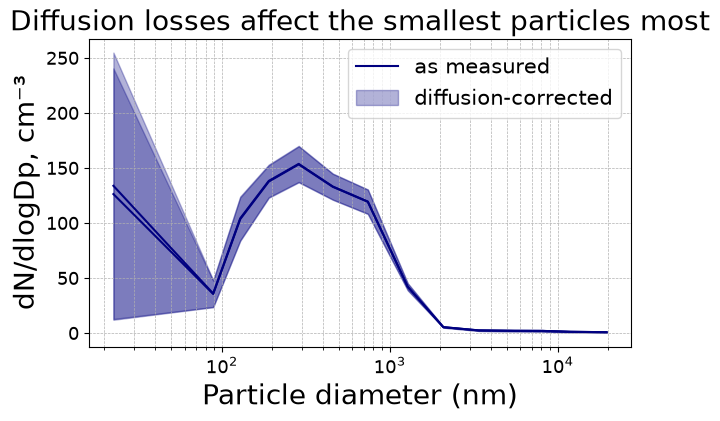
Small particles are lost to the walls of a sampling line by diffusion, so what reaches the instrument understates what was in the air. The correction depends on the tube geometry and the flow through it.
[9]:
corrected = elpi.correct_diffusion_losses(
    D_tube=0.004,   # inner diameter [m]
    L=1.5,          # tube length [m]
    Q=1.0,          # flow [L/min]
    T=293,          # temperature [K]
    P=101300,       # pressure [Pa]
    inplace=False,
)

ratio = corrected.total_concentration.mean() / elpi.total_concentration.mean()
print(f"mean concentration increased by a factor {ratio:.3f}")
mean concentration increased by a factor 1.017
The correction only ever increases concentrations, and most strongly at the small end where diffusion is fastest. Compare the two distributions to see where it acts:
[10]:
import matplotlib.pyplot as plt

fig, ax = plt.subplots(figsize=(7, 4))
elpi.plot_psd(ax=ax, activities=["All data"])
corrected.plot_psd(ax=ax, activities=["All data"])
ax.legend(["as measured", "diffusion-corrected"])
ax.set_title("Diffusion losses affect the smallest particles most")
[10]:
Text(0.5, 1.0, 'Diffusion losses affect the smallest particles most')
PM fractions
pm_calc integrates the distribution below a cut diameter. Results are cached in .extra_data, so asking twice costs nothing.
[11]:
elpi.pm_calc(dtype="dM", PM=2.5)
elpi.pm_calc(dtype="dM", PM=4.2)
elpi.pm_calc(dtype="dM", PM=10)

[c for c in elpi.extra_data.columns if c.startswith("PM")]
[11]:
['PM10', 'PM2.5', 'PM1', 'PM4.2']
lower_lim gives a band instead of a cumulative fraction — the mass between two diameters rather than everything below one.
[12]:
elpi.pm_calc(dtype="dM", PM=4.0, lower_lim=1.0)

[c for c in elpi.extra_data.columns if c.startswith("PM")]
[12]:
['PM10', 'PM2.5', 'PM1', 'PM4.2', 'PM1-4']
The same integration is available for number, surface and volume by changing dtype — dN gives PN, dS gives PS, dV gives PV. These are the metric names accepted by summarize_exposure, see 4 — Statistics and exposure.
Next: 7 — Combining datasets.